There cannot be a greater mistake than that of looking superciliously upon practical applications of science. The life and soul of science is its practical application.
In the first four chapters, we have concentrated on applications of the first and second laws to simple systems (e.g., turbine, throttle). The constraints imposed by the second law should be clear. In this chapter, we show how the analyses we have developed for one or two operations at a time can be assembled into complex processes. In this way, we provide several specific examples of ways that operations can be connected to create power cycles, refrigeration cycles, and liquefaction cycles. We can consider these processes as paradigms for general observations about energy and entropy constraints.
Chapter Objectives: You Should Be Able to…
1. Write energy and entropy balances around multiple pieces of equipment using correct notation including mass flow rates.
2. Simplify energy balances by recognizing when streams have the same properties (e.g., splitter) or flow rates (heat exchanger inlet/outlet).
3. Apply the correct strategy for working through a power cycle with multiple reheaters and feedwater preheaters.
4. For ordinary vapor compression cycles, locate condenser/evaporator P or T given one or the other and plot the process outlet and P-H diagram.
5. Successfully approach complex processes by simplifying the E-balance and S-balance, solving for unknowns.
5.1. The Carnot Steam Cycle
We saw in Example 4.4 on page 145 how a Carnot cycle could be set up using steam as a working fluid. The addition of heat at constant temperature and the macroscopic definition of entropy establish a correspondence between temperature and heat addition/removal. Steam is especially well suited for isothermal heat exchange because boiling and condensation are naturally isothermal and exchange large amounts of heat. To review, we could plot this cycle in T-S coordinates and envision a flow process with a turbine to produce work during adiabatic expansion and some type of compressor for the adiabatic compression as shown in Fig. 5.1. The area inside the P-V cycle represents the work done by the gas in one cycle, and the area enclosed by the T-S path is equal to the net intake of energy as heat by the gas in one cycle.

Figure 5.1. Illustration of a Carnot cycle based on steam in T-S coordinates.
The Carnot cycle has a major advantage over other cycles. It operates at the highest temperature available for as long as possible, reducing irreversibilities at the boundary because the system approaches the reservoir temperature during the entire heat transfer. In contrast, other cycles may only approach the hot reservoir temperature for a short segment of the heat transfer. A similar argument holds regarding the low temperature reservoir. Unfortunately, it turns out that it is impossible to make full use of the advantages of the Carnot cycle in practical applications. When steam is used as the working fluid, the Carnot cycle is impractical for three reasons: 1) It is impractical to stay inside the phase envelope because higher temperatures correlate with higher pressure. Higher pressures lead to smaller heat of vaporization to absorb heat. Since the critical point of water is only ~374°C, substantially below the temperatures from combustion, the temperature gradient between a fired heater and the steam would be large; 2) expanding saturated vapor to low-quality (very wet) steam damages turbine blades by rapid erosion due to water droplets; 3) compressing a partially condensed fluid is much more complex than compressing an entirely condensed liquid. Therefore, most power plants are based on modifications of the Rankine cycle, discussed below. Nevertheless, the Carnot cycle is so simple that it provides a useful estimate for checking results from calculations regarding other cycles.
5.2. The Rankine Cycle
In a Rankine cycle, the vapor is superheated before entering the turbine. The superheat is adjusted to avoid the turbine blade erosion from low-quality steam. Similarly, the condenser completely reduces the steam to a liquid that is convenient for pumping.
In Fig. 5.2, state 4′ is the outlet state for a reversible adiabatic turbine. We use the prime (′) to denote a reversible outlet state as in the previous chapter. State 4 is the actual outlet state which is calculated by applying the efficiency to the enthalpy change.
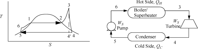
Figure 5.2. Rankine cycle.
![]() The prime denotes a reversible outlet state.
The prime denotes a reversible outlet state.

Because a real turbine always generates entropy, state 4 will always be to the right of 4′ on a T-S diagram. States 4 and 4′ can be inside or outside the phase envelope. Efficiencies are greater if state 4 is slightly inside the phase envelope because the enthalpy change will be larger for the same pressure drop due to the large enthalpy of vaporization; however, to avoid turbine blade damage, quality is kept above 90% in most cases.
Note in Fig. 5.2 that the superheater between the boiler and the turbine is not drawn, and only a single unit is shown. In actual power plants, separate superheaters are used; however, for the sake of simplicity in our discussions the boiler/superheater steam generator combination will be represented by a single unit in the schematic.
![]() Most plants will have separate boilers and superheaters. We show just a boiler for simplicity.
Most plants will have separate boilers and superheaters. We show just a boiler for simplicity.
Turbine calculation principles were covered in the last chapter. Now we recognize that the net work is the sum of the work for the turbine and pump and that some of the energy produced by the turbine is needed for the pump. In general, the thermal efficiency is given by:

The boiler input can be calculated directly from the enthalpy out of the pump and the desired turbine inlet. The key steps are illustrated in Example 5.1.
A power plant uses the Rankine cycle. The turbine inlet is 500°C and 1.4 MPa. The outlet is 0.01 MPa. The turbine has an efficiency of 85% and the pump has an efficiency of 80%. Determine:
a. The work done by the turbine (kJ/kg)
b. The work done by the pump, the heat required, and the thermal efficiency;
c. The circulation rate to provide 1 MW net power output.
Solution
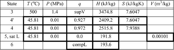
We will refer to Fig. 5.2 for stream numbers. The recommended method for solving process problems is to establish a table to record values as they are determined. In this text we will show values in the tables with bold borders if they have been determined by balance calculations. The turbine outlet can be read from the temperature table without interpolation. Cells with standard borders refer to properties determined directly from the problem statement
![]() Boldfaced table cells show calculations that were determined by balances. We follow this convention in the following examples.
Boldfaced table cells show calculations that were determined by balances. We follow this convention in the following examples.
Because the turbine inlet has two state variables specified, the remainder of the state properties are found from the steam tables and tabulated in the property table. We indicate a superheated vapor with “supV” compressed liquid with “compL.”
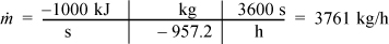
a. Stepping forward across the turbine involves the same specifications as part (c) of Example 4.13 on page 168. The properties from 4 and 4′ are transferred from that example to the property table. The work done is –959 kJ/kg.
b. The outlet of the condenser is taken as saturated liquid at the specified pressure, and those values are entered into the table. We must calculate ![]() and
and ![]() . So we need H6 and WS,pump which are determined by calculating the adiabatic work input by the pump to increase the pressure from state 5. Although the reversible calculation for the pump is isentropic, we may apply Eqn. 2.61 without direct use of entropy, and then correct for efficiency. For the pump,
. So we need H6 and WS,pump which are determined by calculating the adiabatic work input by the pump to increase the pressure from state 5. Although the reversible calculation for the pump is isentropic, we may apply Eqn. 2.61 without direct use of entropy, and then correct for efficiency. For the pump,
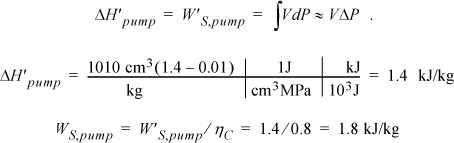
Thus, the work of the pump is small, resulting in H6 = 191.8 + 1.8 = 193.6 kJ/kg. The net work is W’S,net = –959.0 + 1.8 = 957.2 kJ/kg. The only source of heat for the cycle is the boiler/superheater. All of the heat input is at the boiler/superheater. The energy balance gives QH = (H3 – H6) = 3281.2 kJ/kg. The thermal efficiency is
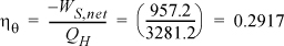
If we neglected the pump work, the efficiency would 29.23%. Note that the pump work has only a small effect on the thermal efficiency but is included for theoretical rigor.
c. For 1 MW capacity, ![]() , the circulation rate is
, the circulation rate is
The cycle in Fig. 5.2 is idealized from a real process because the inlet to the pump is considered saturated. In a real process, it will be subcooled to avoid difficulties (e.g., cavitation1) in pumping. In fact, real processes will have temperature and pressure changes along the piping between individual components in the schematic, but these changes will be considered negligible in the Rankine cycle and all other processes discussed in the chapter, unless otherwise stated. These simplifications allow focus on the most important concepts, but the simplifications would be reconsidered in a detailed process design.
5.3. Rankine Modifications
Two modifications of the Rankine cycle are in common use to improve the efficiency. A Rankine cycle with reheat increases the boiler pressure but keeps the maximum temperature approximately the same. The maximum temperatures of the boilers are limited by corrosion concerns. This modification uses a two-stage turbine with reheat in-between. An illustration of the modified cycle is shown in Fig. 5.3. Crudely, adding multiple stages with reheat leads to the maximum temperature being applied as much as possible, while avoiding extremely wet steam during expansion. This moves the process efficiency in the direction of a Carnot cycle. The implication of this modification is shown in Example 5.2.
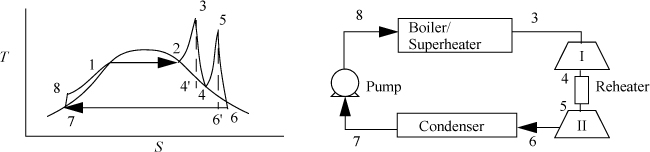
Figure 5.3. Rankine cycle with reheat.
Example 5.2. A Rankine cycle with reheat
Consider a modification of Example 5.1. If we limit the process to a 500°C boiler/superheater with reheat, we can develop a new cycle to investigate an improvement in efficiency and circulation rate. Let us operate a cycle utilizing two reversible turbines with ηE = 0.85 and a pump with ηC = 0.8. Let the feed to the first turbine be steam at 500°C and 6 MPa. Let the feed to the second stage be 1.4 MPa and 500°C (the same as Example 5.1). Determine the improvement in efficiency and circulation rate relative to Example 5.1.
Solution
Refer to Fig. 5.3 for stream numbers. First, let us find state 3. The inlet state values are entered in the table. P4 = P5 because we neglect the heat exchanger pressure drop. Upon expansion through the first reversible turbine, we look at the SsatV at 1.4 MPa and find it lower that S4’. Therefore, the reversible state is superheated. Using {S,P} to find H,

Correcting for efficiency,
ΔHI = WS, I = 0.85(3001.2 – 3423.1) = 0.85(–421.9) = –358.6 kJ/kg
H4 = 3423.1 – 358.6 = 3064.5 kJ/kg
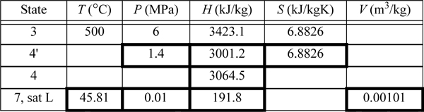
State 5 was used in Example 5.1 (as state 3). Solving the energy balance for the reheater,
Qreheat = (H5 – H4) = 3474.8 – 3064.5 = 410.3 kJ/kg
Turbine II was analyzed in Example 5.1. We found WS,II = –959.0 kJ/kg and the total work output is WS,turbines = (–358.6 –959.0) = –1317.6 kJ/kg. The pump must raise the pressure to 6 MPa. Using Eqn. 2.61, and correcting for efficiency,

State 7 is the same as state 5 in Example 5.1 and has been tabulated in the property table. H8 = H7 + WS,pump = 191.8 + 7.6 = 199.4 kJ/kg. The net work is thus
WS, net = –1317.6 + 7.6 = –1310 kJ/kg
The heat for the boiler/superheater is given by Qb/s = H3 – H8 = 3423.1 – 199.4 = 3223.7 kJ/kg.
The thermal efficiency is
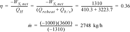
The efficiency has improved by ![]() , and the circulation rate has been decreased by 27%.
, and the circulation rate has been decreased by 27%.
Leave a Reply