The problem solving tools on the desktop that were used by engineers prior to the introduction of the handheld calculators (i.e., before 1970) are shown in Figure 1-1. Most calculations were carried out using the slide rule. This required carrying out each arithmetic operation separately and writing down the results of such operations. The highest precision of such calculations was to three decimal digits at most. If a calculational error was detected, then all the slide rule and arithmetic calculations had to be repeated from the point where the error occurred. The results of the calculations were typically typed, and hand-drawn graphs were often prepared. Temperature- and/or composition-dependent thermodynamic and physical properties that were needed for problem solving were represented by graphs and nomographs. The values were read from a straight line passed by a ruler between two points. The highest precision of the values obtained using this technique was only two decimal digits. All in all, “manual” problem solving was a tedious, time-consuming, and error-prone process.

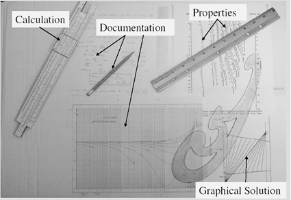
Figure 1-1. The Engineer’s Problem Solving Tools Prior to 1970

During the slide rule era, several techniques were developed that enabled solving realistic problems using the tools that were available at that time. Analytical (closed form) solutions to the problems were preferred over numerical solutions. However, in most cases, it was difficult or even impossible to find analytical solutions. In such cases, considerable effort was invested to manipulate the model equations of the problem to bring them into a solvable form. Often model simplifications were employed by neglecting terms of the equations which were considered less important. “Short-cut” solution techniques for some types of problems were also developed where a complex problem was replaced by a simple one that could be solved. Graphical solution techniques, such as the McCabe-Thiele and Ponchon-Savarit methods for distillation column design, were widely used.

After digital computers became available in the early 1960’s, it became apparent that computers could be used for solving complex engineering problems. One of the first textbooks that addressed the subject of numerical solution of problems in chemical engineering was that by Lapidus.^[3] The textbook by Carnahan, Luther and Wilkes^[4] on numerical methods and the textbook by Henley and Rosen^[5] on material and energy balances contain many example problems for numerical solution and associated mainframe computer programs (written in the FORTRAN programming language). Solution of an engineering problem using digital computers in this era included the following stages: (1) derive the model equations for the problem at hand, (2) find the appropriate numerical method (algorithm) to solve the model, (3) write and debug a computer language program (typically FORTRAN) to solve the problem using the selected algorithm, (4) validate the results and prepare documentation.

Problem solving using numerical methods with the early digital computers was a very tedious and time-consuming process. It required expertise in numerical methods and programming in order to carry out the 2nd and 3rd stages of the problem-solving process. Thus the computer use was justified for solving only large-scale problems from the 1960’s through the mid 1980’s.

Mathematical software packages started to appear in the 1980’s after the introduction of the Apple and IBM personal computers. POLYMATH version 1.0, the software package which is extensively used in this book, was first published in 1984 for the IBM personal computer.

Introduction of mathematical software packages on mainframe and now personal computers has considerably changed the approach to problem solving. Figure 1-2 shows a flow diagram of the problem-solving process using such a package. The user is responsible for the preparation of the mathematical model (a complete set of equations) of the problem. In many cases the user will also need to provide data or correlations of physical properties of the compounds involved. The complete model and data set must be fed into the mathematical software package. It is also the user’s responsibility to categorize the problem type. The problem category will determine the type of numerical algorithm to be used for the solution. This issue will be discussed in detail in the next section.

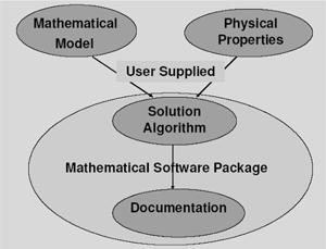
Figure 1-2. Problem Solving with Mathematical Software Packages

The mathematical software package will then solve the problem using the selected numerical technique. The results obtained together with the model definition can serve as partial or complete documentation of the problem and its solution.

Categorizing Problems According to the Solution Technique Used

Mathematical software packages contain various tools for problem solving. In order to match the tool to the problem in hand, you should be able to categorize the problem according to the numerical method that should be used for its solution. The discussion in this section details the various categories for which representative examples are included in the book. Note that the study of the following categories (a) through (e) is highly recommended prior to using Chapters 7 through 14 of this book that are associated with particular subject areas. Categories (f) through (n) are advanced topics that should be reviewed prior to advanced problem solving.