Flow in Noncircular Ducts

The cross section of a pipe is most frequently circular, but other shapes may be encountered. For example, the rectangular cross section of many domestic hotair heating ducts should be apparent to most people living in the United States. The situation for a horizontal duct is illustrated in Fig. 3.14; the cross-sectional shape is quite arbitrary—it doesn’t have to be rectangular as shown—as long as it is uniform at all locations. There, A is the cross-sectional area and P is the wetted perimeter—defined as the length of wall that is actually in contact with the fluid. For the flow of a gas, P will always be the length of the complete periphery of the duct; for liquids, however, it will be somewhat less than the periphery if the liquid has a free surface and incompletely fills the total cross section.

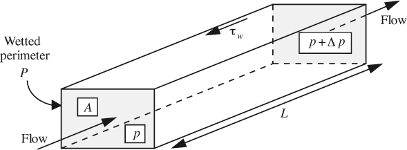
Fig. 3.14 Flow in a duct of noncircular cross section.

If τ_w is the wall shear stress and there is a pressure drop –Δp over a length L, a momentum balance in the direction of flow yields:

The pressure drop is therefore:

Thus, the equation for the pressure drop is identical with that of Eqn. (3.33) for a circular pipe provided that D is replaced by the hydraulic mean diameter D_e, defined by:

The reader may wish to check that D_e = D for a circular duct. Following similar lines as those used previously, the frictional dissipation per unit mass can be deduced as:

and this expression can then be employed for inclined ducts of noncircular cross section.

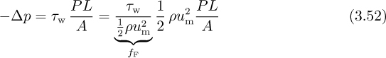
Steady flow in open channels. A similar treatment follows for a liquid flowing steadily down a channel inclined at an angle θ to the horizontal, such as a river or irrigation ditch, shown in Fig. 3.15. Again, as long as the cross section is uniform along the channel, it can be quite arbitrary in shape, not necessarily rectangular. The driving force is now gravity, there being no variation of pressure because the free surface is uniformly exposed to the atmosphere.

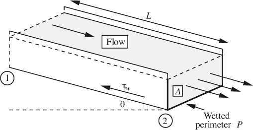
Fig. 3.15 Flow in an open channel.

If the wetted perimeter is again P and the cross-sectional area occupied by the liquid is A, a steady-state momentum balance in the direction of flow gives:

Noting that:

division of Eqn. (3.56) by –ρA gives:

in which the second term can be rearranged as:

Comparison with the overall energy balance:

gives the frictional dissipation per unit mass as:

which has exactly the same form as Eqns. (3.54) and (3.55).

---

Example 3.6—Flow in an Irrigation Ditch

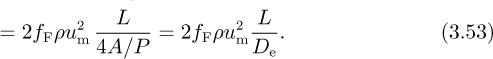
The irrigation ditch shown in Fig. E3.6 has a cross section that is 6 ft wide × 6 ft deep. It conveys water from location 1 to location 2, between which there is a certain drop in elevation.

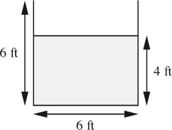
Fig. E3.6 Cross section of irrigation ditch.

With a flow rate of Q = 72 ft³/s of water, the ditch is filled to a depth of 4 ft. If the same ditch, transporting water between the same two locations, were completely filled to a depth of 6 ft, by what percentage would the flow rate increase? Start by applying the overall energy balance between points 1 and 2, and assume that the friction factor remains constant.

Solution

Apply the energy equation between two points separated by a distance L:

or,

Whether the ditch is filled to 4 ft or 6 ft, all quantities in Eqn. (E3.6.1) remain the same except u_m and D_e, so that:

in which c is a factor that incorporates everything that remains constant.

Case 1. When the ditch is filled to a depth of only 4 ft, the hydraulic mean diameter is:

But the mean velocity is:

so that the value of the constant in Eqn. (E3.6.2) is:

Case 2. When the ditch is filled to a depth of 6 ft, the hydraulic mean diameter is:

From Eqns. (E3.6.2) and (E3.6.5), the mean velocity is:

so that the flow rate is now:

The percentage increase in flow rate is therefore:

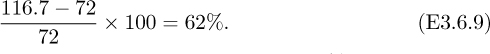
Thus, the increase in flow rate is somewhat more than the 50% increase in the depth of water. The reason is that the increased area for flow is accompanied by a somewhat lower increase in the length of the wetted perimeter.

---

Pressure drop across pipe fittings. A variety of auxiliary hardware such as valves and elbows is associated with most piping installations. These fittings invariably cause the flow to deviate from its normal straight course and hence induce additional turbulence and frictional dissipation. Indeed, the resulting additional pressure drop is sometimes comparable to that in the pipeline itself.

The basic procedure is to recognize that the fitting causes an additional pressure drop that would be produced by a certain length of pipe into which the fitting is introduced. Therefore, we substitute for the fitting an extra contribution to the length of the pipe, based on the equivalent length (L/D)_e of the fitting. For example, referring to Table 3.4, three standard 90° elbows in a 6–in.-diameter line cause a pressure drop that is equivalent to an extra 45 ft of pipe.

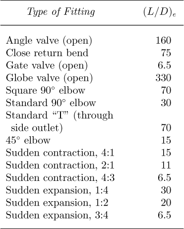
Table 3.4 Equivalent Lengths of Pipe Fittings^9,10

⁹ See for example, G.G. Brown et al., Unit Operations, Wiley & Sons, New York, 1950, p. 140.

¹⁰ For sudden expansions and contractions, the diameter ratio is given in Table 3.4; also, the equivalent length in these cases is based on the smaller diameter.

The gate valve uses a retractable circular plate that normally has one of two extreme positions: (a) complete obstruction of the flow, or (b) essentially no obstruction. The gate valve cannot be used for fine control of the flow rate, for which the globe or needle valve, with an adjustable plug or needle partly obstructing a smaller orifice, is more effective.

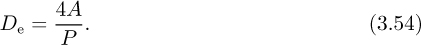
Laminar and turbulent velocity profiles. The parabolic velocity profile already encountered in laminar flow in a pipe is again illustrated on the left of Fig. 3.16. On the right, we see for the first time the general shape of the velocity profile for turbulent flow. Chapter 9 shows that although in turbulent flow the velocities exhibit random fluctuations, it is still possible to work in terms of a time-averaged axial velocity. For simplicity at this stage, we shall still use u to denote such a quantity, although in Chapter 9 it will be replaced with a symbol such as .

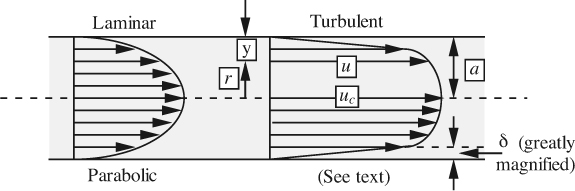
Fig. 3.16 Laminar and turbulent velocity profiles.

In addition to the generally higher velocities, note that the overall turbulent velocity profile consists of two profoundly different zones:

1. A very thin region, known as the laminar sublayer, in which turbulent effects are essentially absent, the shear stress is virtually constant, and there is an extremely steep velocity gradient. The following equation is derived in Section 9.7 for the thickness δ of the laminar sublayer relative to the pipe diameter D as a function of the Reynolds number in the pipe:

Observe that the laminar sublayer becomes thinner as the Reynolds number increases, because the greater intensity of turbulence extends closer to the wall.

2. A turbulent core, which extends over nearly the whole cross section of the pipe. Here, the velocity profile is relatively flat because rapid turbulent radial momentum transfer tends to “iron out” any differences in velocity. A representative equation for the ratio of the velocity u at a distance y from the wall to the centerline velocity u_c is:

in which n in the exponent varies somewhat with the Reynolds number, as in Table 3.5. For n = 1/7, Eqn. (3.63) is plotted in Fig. 9.11.

Table 3.5 Exponent n for Equation (3.63)¹¹

¹¹ H. Schlichting, Boundary-Layer Theory, McGraw-Hill, New York, 1955, p. 403.