S = k ln W
L. Boltzmann
We have discussed energy balances and the fact that friction and velocity gradients cause the loss of useful work. It would be desirable to determine maximum work output (or minimum work input) for a given process. Our concern for accomplishing useful work inevitably leads to a search for what might cause degradation of our capacity to convert any form of energy into useful work. As an example, isothermally expanding an ideal gas from Vi to 2Vi can produce a significant amount of useful work if carried out reversibly, or possibly zero work if carried out irreversibly. If we could understand the difference between these two operations, we would be well on our way to understanding how to minimize wasted energy in many processes. Inefficiencies are addressed by the concept of entropy.
Entropy provides a measure of the disorder of a system. As we will see, increased “disorder of the universe” leads to reduced capability for performing useful work. This is the second law of thermodynamics. Conceptually, it seems reasonable, but how can we define “disorder” mathematically? That is where Boltzmann showed the way:
S = klnW
where S is the entropy, W is the number of ways of arranging the molecules given a specific set of independent variables, like T and V; k is known as Boltzmann’s constant.
For example, there are more ways of arranging your socks around the entire room than in a drawer, basically because the volume of the room is larger than that of the drawer. We will see that ΔS = Nkln(V2/V1) in this situation, where N is the number of socks and Nk = nR, where n is the number of moles, V is the volume, and R is the gas constant. In Chapter 1, we wrote Uig = 1.5NkT without thinking much about who Boltzmann was or how his constant became so fundamental to the molecular perspective. This connection between the molecular and macroscopic scales was Boltzmann’s major contribution.
Chapter Objectives: You Should Be Able to…
1. Explain entropy changes in words and with numbers at the microscopic and macroscopic levels. Typical explanations involve turbines, pumps, heat exchangers, mixers, and power cycles.
2. Simplify the complete entropy balance to its most appropriate form for a given situation and solve for the productivity of a reversible process.
3. Sketch and interpret T-S, T-V, H-S, and P-H diagrams for typical processes.
4. Use inlet and outlet conditions and efficiency to determine work associated with turbines/compressors.
5. Determine optimum work interactions for reversible processes as benchmarks for real systems.
6. Sketch and interpret T-S, T-V, H-S, and P-H diagrams for typical processes.
4.1. The Concept of Entropy
Chapters 2 and 3 showed the importance of irreversibility when it comes to efficient energy transformations. We noted that prospective work energy was generally dissipated into thermal energy (stirring) when processes were conducted irreversibly. If we only had an “irreversibility meter,” we could measure the irreversibility of a particular process and design it accordingly. Alternatively, we could be given the efficiency of a process relative to a reversible process and infer the magnitude of the irreversibility from that. For example, experience might show that the efficiency of a typical 1000 kW turbine is 85%. Then, characterizing the actual turbine would be simple after solving for the reversible turbine (100% efficient).
In our initial encounters, entropy generation provides this measure of irreversibility. Upon studying entropy further, however, we begin to appreciate its broader implications. These broader implications are especially important in the study of multicomponent equilibrium processes, as discussed in Chapters 8–16. In Chapters 5–7, we learn to appreciate the benefits of entropy being a state property. Since its value is path independent, we can envision various ways of computing it, selecting the path that is most convenient in a particular situation.
Entropy may be contemplated microscopically and macroscopically. The microscopic perspective favors the intuitive connection between entropy and “disorder.” The macroscopic perspective favors the empirical approach of performing systematic experiments, searching for a unifying concept like entropy. Entropy was initially conceived macroscopically, in the context of steam engine design. Specifically, the term “entropy” was coined by Rudolf Clausius from the Greek for transformation.1 To offer students connections with the effect of volume (for gases) and temperature, this text begins with the microscopic perspective, contemplating the detailed meaning of “disorder” and then demonstrating that the macroscopic definition is consistent.
![]() Entropy is a useful property for determining maximum/minimum work.
Entropy is a useful property for determining maximum/minimum work.
Rudolf Julius Emanuel Clausius (1822–1888), was a German physicist and mathematician credited with formulating the macroscopic form of entropy to interpret the Carnot cycle and developed the second law of thermodynamics.
To appreciate the distinction between the two perspectives on entropy, it is helpful to define the both perspectives first. The macroscopic definition is especially convenient for solving problems process problems, but the connection between this definition and disorder is not immediately apparent.
Macroscopic definition—Intensive entropy is a state property of the system. For a differential change in state of a closed simple system (no internal temperature gradients or composition gradients and no internal rigid, adiabatic, or impermeable walls),2 the differential entropy change of the system is equal to the heat absorbed by the system along a reversible path divided by the absolute temperature of the system at the surface where heat is transferred.
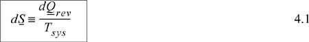
where dS is the entropy change of the system. We will later show that this definition is consistent with the microscopic definition.
Microscopic definition—Entropy is a measure of the molecular disorder of the system. Its value is related to the number of microscopic states available at a particular macroscopic state. Specifically, for a system of fixed energy and number of particles, N,
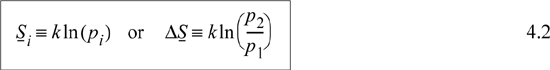
where pi is the number of microstates in the ith macrostate, k = R/NA. We define microstates and macrostates in the next section.
The microscopic perspective is directly useful for understanding how entropy changes with volume (for a gas), temperature, and mixing. It simply states that disorder increases when the number of possible arrangements increases, like the socks and drawers mentioned in the introduction. Similarly, molecules redistribute themselves when a valve is opened until the pressures have equilibrated. From the microscopic approach, entropy is a specific mathematical relation related to the number of possible arrangements of the molecule. Boltzmann showed that this microscopic definition is entirely consistent with the macroscopic property inferred by Rudolf Clausius. We will demonstrate how the approaches are equivalent.
Entropy is a difficult concept to understand, mainly because its influence on physical situations is subtle, forcing us to rely heavily on the mathematical definition. We have ways to try to make some physical connection with entropy, and we will discuss these to give you every opportunity to develop a sense of how entropy changes. Ultimately, you must reassure yourself that entropy is defined mathematically, and like enthalpy, can be used to solve problems even though our physical connection with the property is occasionally less than satisfying.
In Section 4.2, the microscopic definition of entropy is discussed. On the microscopic scale, S is influenced primarily by spatial arrangements (affected by volume and mixing), and energetic arrangements (occupation) of energy levels (affected by temperature). We clarify the meaning of the microscopic definition by analyzing spatial distributions of molecules. To make the connection between entropy and temperature, we outline how the principles of volumetric distributions extend to energetic distributions. In Section 4.3, we introduce the macroscopic definition of entropy and conclude with the second law of thermodynamics.
![]() The microscopic approach to entropy is discussed first, then the macroscopic approach is discussed.
The microscopic approach to entropy is discussed first, then the macroscopic approach is discussed.
The second law is formulated mathematically as the entropy balance in Section 4.4. In this section we demonstrate how heat can be converted into work (as in an electrical power plant). However, the maximum thermal efficiency of the conversion of heat into work is less than 100%, as indicated by the Carnot efficiency. The thermal efficiency can be easily derived using entropy balances. This simple but fundamental limitation on the conversion of heat into work has a profound impact on energy engineering. Section 4.5 is a brief section, but makes the key point that pieces of an overall process can be reversible, even while the overall process is irreversible.
In Section 4.6 we simplify the entropy balance for common process equipment, and then use the remaining sections to demonstrate applications of system efficiency with the entropy balance. Overall, this chapter provides an understanding of entropy which is essential for Chapter 5 where entropy must be used routinely for process calculations.
4.2. The Microscopic View of Entropy
Probability theory is nothing but common sense reduced to calculation.
LaPlace
To begin, we must recognize that the disorder of a system can change in two ways. First, disorder occurs due to the physical arrangement (distribution) of atoms, and we represent this with the configurational entropy.3 There is also a distribution of kinetic energies of the particles, and we represent this with the thermal entropy. For an example of kinetic energy distributions, consider that a system of two particles, one with a kinetic energy of 3 units and the other of 1 unit, is microscopically distinct from the same system when they both have 2 units of kinetic energy, even when the configurational arrangement of atoms is the same. This second type of entropy is more difficult to implement on the microscopic scale, so we focus on the configurational entropy in this section.4
![]() Configurational entropy is associated with spatial distribution. Thermal entropy is associated with kinetic energy distribution.
Configurational entropy is associated with spatial distribution. Thermal entropy is associated with kinetic energy distribution.
Entropy and Spatial Distributions: Configurational Entropy
Given N molecules and M boxes, how can these molecules be distributed among the boxes? Is one distribution more likely than another? Consideration of these issues will clarify what is meant by microstates and macrostates and how entropy is related to disorder. Our consideration will focus on the case of distributing particles between two boxes.
![]() Distinguishability of particles is associated with microstates. Indistinguishability is associated with macrostates.
Distinguishability of particles is associated with microstates. Indistinguishability is associated with macrostates.
First, let us suppose that we distribute N = 2 ideal gas5 molecules in M = 2 boxes, and let us suppose that the molecules are labeled so that we can identify which molecule is in a particular box. We can distribute the labeled molecules in four ways, as shown in Fig. 4.1. These arrangements are called microstates because the molecules are labeled. For two molecules and two boxes, there are four possible microstates. However, a macroscopic perspective makes no distinction between which molecule is in which box. The only macroscopic characteristic that is important is how many particles are in a box, rather than which particle is in a certain box. For macrostates, we just need to keep track of how many particles are in a given box, not which particles are in a given box. It might help to think about connecting pressure gauges to the boxes. The pressure gauge could distinguish between zero, one, and two particles in a box, but could not distinguish which particles are present. Therefore, microstates α and δ are different macrostates because the distribution of particles is different; however, microstates β and γ give the same macrostate. Thus, from our four microstates, we have only three macrostates.

Figure 4.1. Illustration of configurational arrangements of two molecules in two boxes, showing the microstates. Not that β and γ would have the same macroscopic value of pressure.
To find out which arrangement of particles is most likely, we apply the “principle of equal a priori probabilities.” This “principle” states that all microstates of a given energy are equally likely. Since all of the states we are considering for our non-interacting particles are at the same energy, they are all equally likely.6 From a practical standpoint, we are interested in which macrostate is most likely. The probability of a macrostate is found by dividing the number of microstates in the given macrostate by the total number of microstates in all macrostates as shown in Table 4.1. For our example, the probability of the first macrostate is 1/4 = 0.25. The probability of the evenly distributed state is 2/4 = 0.5. That is, one-third of the macrostates possess 50% of the probability. The “most probable distribution” is the evenly distributed case.
Table 4.1. Illustration of Macrostates for Two Particles and Two Boxes

What happens when we consider more particles? It turns out that the total number of microstates for N particles in M boxes is MN, so the counting gets tedious. For five particles in two boxes, the calculations are still manageable. There will be two microstates where all the particles are in one box or the other. Let us consider the case of one particle in box A and four particles in box B. Recall that the macrostates are identified by the number of particles in a given box, not by which particles are in which box. Therefore, the five microstates for this macrostate appear as given in Table 4.2(a).
Table 4.2. Microstates for the Second and Third Macrostates for Five Particles Distributed in Two Boxes

The counting of microstates for putting two particles in box A and three in box B is slightly more tedious, and is shown in Table 4.2(b). It turns out that there are 10 microstates in this macrostate. The distributions for (three particles in A) + (two in B) and for (four in A) + (one in B) are like the distributions (two in A) + (three in B), and (one in A) + (four in B), respectively. These three cases are sufficient to determine the overall probabilities. There are MN = 25 = 32 microstates total summarized in the table below.

Note now that one-third of the macrostates (two out of six) possess 62.5% of the microstates. Thus, the distribution is now more peaked toward the most evenly distributed states than it was for two particles where one-third of the macrostates possessed 50% of the microstates. This is one of the most important aspects of the microscopic approach. As the number of particles increases, it won’t be long before 99% of the microstates are in one-third of the macrostates. The trend will continue, and increasing the number of particles further will quickly yield 99% of the microstates in that one-tenth of the macrostates. In the limit as N→∞ (the “thermodynamic limit”), virtually all of the microstates are in just a few of the most evenly distributed macrostates, even though the system has a very slight finite possibility that it can be found in a less evenly distributed state. Based on the discussion, and considering the microscopic definition of entropy (Eqn. 4.2), entropy is maximized at equilibrium for a system of fixed energy and total volume.7
Leave a Reply