Energy Balances for Composite Systems

A theory is the more impressive the greater the simplicity of its premises is, the more different kinds of things it relates, and the more extended is its area of applicability. Therefore the deep impression which classical thermodynamics made upon me.

Albert Einstein

Having established the principle of the energy balance for individual systems, it is straightforward to extend the principle to a collection of several individual systems working together to form a composite system. One of the simplest and most enlightening examples is the Carnot cycle which is a benchmark system used to evaluate conversion of heat into work. The principle of the first law is perhaps most powerful when applied from an overall perspective. In other words, it is not necessary to deal with individual operations in order to draw conclusions about the overall system. Clever selections of composite systems or subsystems can then permit valuable insights about key behaviors and where to focus greater analysis. Implementing this overall perspective often requires dealing with multicomponent and reacting systems. For example, calorie counting for dietary needs must consider at least glucose, oxygen, CO₂, and water. It is not necessary at this stage to have a precise estimate of the mixture properties, but the reality of mixed systems must be acknowledged approximately. To illustrate practical implications, we consider distillation systems, reacting systems, and biological systems.

Chapter Objectives: You Should Be Able to…

1. Understand the steps of a Carnot engine and Carnot heat pump.

2. Analyze cycles to compute the work and heat input per cycle.

3. Apply the concepts of constant molar overflow in distillation systems.

4. Apply the concepts of ideal gas mixtures and ideal mixtures to energy balances.

5. Apply mole balances for reacting systems using reaction coordinates for a given feed properly using the stoichiometric numbers for single and multiple reactions.

6. Properly determine the standard heat of reaction at a specified temperature.

7. Use the energy balance properly for a reactive system.

3.1. Heat Engines and Heat Pumps – The Carnot Cycle

In this section we introduce the Carnot cycle as a method to convert heat to work. Many power plants work on the same general principle of using heat to produce work. In a power plant, heat is generated by coal, natural gas, or nuclear energy. However, only a portion of this energy can be used to generate electricity, and the Carnot cycle analysis will be helpful in understanding those limitations. Before we start the analysis, let us define the ratio of net work produced to the heat input as the thermal efficiency using the symbol η_θ:

 Thermal efficiency.

We wish to make the thermal efficiency as large as possible. We prove in the next chapter that the Carnot engine matches the highest thermal efficiency for an engine operating between two isothermal reservoirs. Maximizing thermal efficiency is a design goal that pervades Units I and II. We reconsider the thermal efficiency each time we add a layer of sophistication in our analysis. The concept of entropy in Chapter 4 will help us to generalize from ideal gases to steam or other fluids with available tables and charts. The calculus of classical thermodynamics in Chapter 5 will help to generalize to any substance, making our own tables and charts in Chapters 6–9. Evaluating the thermal efficiency in many situations is a skill that any engineer should have. Chemical engineering embraces a broad scope of … “chemicals.”

The Carnot Engine

The Carnot cycle was conceived by Sadi Carnot as a route to convert heat into work. In the previous chapter, we developed the energy balances and work calculations for reversible isothermal and adiabatic processes. The Carnot engine combines them in a cycle. Consider a piston in the vicinity of both a hot reservoir and a cold reservoir as illustrated in Fig. 3.1. The insulation on the piston may be removed to transfer heat from the hot reservoir during one step of the process, and also removed from the cold side to transfer heat to the cold reservoir during another step of the process. Carnot conceived of the cycle consisting of the steps shown schematically on the P-V diagram beginning from point a. Between points a and b, the gas undergoes an isothermal expansion, absorbing heat from the hot reservoir. From point b to c, the gas undergoes an adiabatic expansion. From point c to d, the gas undergoes an isothermal compression, rejecting heat to the cold reservoir. From point d to a, the gas undergoes an adiabatic compression to return to the initial state.

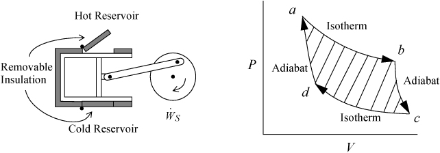
Figure 3.1. Schematic of the Carnot engine, and the Carnot P-V cycle when using a gas as the process fluid.

 The Carnot cycle is one method of constructing a heat engine.

Nicolas Léonard Sadi Carnot (1796–1832) was a French scientist who developed the Carnot cycle to demonstrate the maximum conversion of heat into work.

Let us consider the energy balance for the gas in the piston. Because the process is cyclic and returns to the initial state, the overall change in U is zero. The system is closed, so no flow work is involved. This work performed, W_EC = ∫PdV for the gas, is equal to the work done on the shaft plus the expansion/contraction work done on the atmosphere for each step. By summing the work terms for the entire cycle, the net work done on the atmosphere in a complete cycle is zero since the net atmosphere volume change is zero. Therefore, the work represented by the shaded portion of the P-V diagram is the useful work transferred to the shaft.

You can see from the shaded area in Fig. 3.1 that –W_{S, net} > 0; therefore, since Q_H > 0 and Q_C < 0, . The ratio  is negative, and to maximize η we seek to make Q_C as small in magnitude as possible.

The heat transferred and work performed in the various steps of the process are summarized in Table 3.1. For this calculation we assume the gas within the piston follows the ideal gas law with temperature-independent heat capacities. We calculate reversible changes in the system; thus, we neglect temperature and velocity gradients within the gas (or we perform the process very slowly so that these gradients do not develop).

Table 3.1. Illustration of Carnot Cycle Calculations for an Ideal Gas.^a

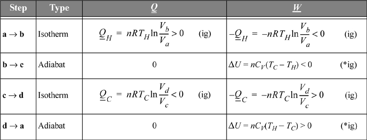
a. The Carnot cycle calculations are shown here for an ideal gas. There are no requirements that the working fluid is an ideal gas, but it simplifies the calculations.

Note: The temperatures T_H and T_C here refer to the hot and cold temperatures of the gas, which are not required to be equal to the temperatures of the reservoirs for the Carnot engine to be reversible. In Chapter 4 we will show that if these temperatures do equal the reservoir temperatures, the work is maximized.

Comparing adiabats b → c and d → a, the work terms must be equal and opposite since the temperature changes are opposite. The temperature change in an adiabatic process is related to the volume change in Eqn. 2.63. In that equation, when the temperature ratio is inverted, the volume ratio is inverted. Therefore, we reason that for the two adiabatic steps, V_b/V_a = V_c/V_d. Using the ratio in the formulas for the isothermal steps, the ratio of heat flows becomes

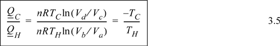
Inserting the ratio of heat flows into Eqn. 3.4 results in the thermal efficiency.

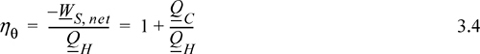
 The thermal efficiency of a heat engine is determined by the upper and lower operating temperatures of the engine.

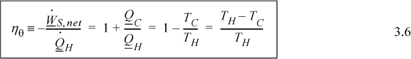
You must use absolute temperature when applying Eqn. 3.6. We can skip the conversion to absolute temperature in the numerator of the last term because the subtraction means that the 273.15 (for units of K) in one term is canceled by the other. There is no such cancellation in the denominator.

Eqn. 3.6 indicates that we cannot achieve η_θ = 1 unless the temperature of the hot reservoir becomes infinite or the temperature of the cold reservoir approaches 0 K. Such reservoir temperatures are not practical for real applications. For real processes, we typically operate between the temperature of a furnace and the temperature of cooling water. For a typical power-plant cycle based on steam as the working fluid, these temperatures might be 900 K for the hot reservoir and 300 K for the cold reservoir, so the maximum thermal efficiency for the process is near 67%, theoretically. Most real power plants operate with thermal efficiencies closer to 30% to 40% owing to inherent inefficiencies in real processes.

Perspective on the Heat Engine

The Carnot cycle provides a quick and convenient guideline for processes that seek to convert heat flow into work. The striking conclusion we will prove in Chapter 4 is that it is impossible to convert all of the heat flow from the hot reservoir into work at reasonable temperatures. From an overall perspective, the detailed steps of the Carnot engine can be ignored. The amount of work is given by Eqn. 3.6. We can simply state that heat comes in, heat goes out, and the difference is the net work. This situation is represented by Fig. 3.2(a). As an alternate perspective, any process with a finite temperature gradient should produce work. If it does not, then it must be irreversible, and “wasteful.” This situation is represented by Fig. 3.2(b). These observations are similar to previous statements about gradients and irreversibility, but Eqn. 3.6 establishes a quantitative connection between the temperature difference and the reversible work possible.

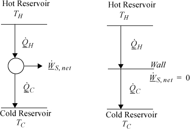
Figure 3.2. The price of irreversibility. (a) Overall energy balance perspective for the reversible heat engine. (b) Zero work production in a temperature gradient without a heat engine, Q_H = Q_C.