All the effects of nature are only the mathematical consequences of a small number of immutable laws.
P.-S. LaPlace
Maxwell’s relations make it clear that changes in any one variable can be represented as changes in some other pair of variables. In chemical processes, we are often concerned with the changes of enthalpy and entropy as functions of temperature and pressure. As an example, recall the operation of a reversible turbine between some specified inlet conditions of T and P and some specified outlet pressure. Using the techniques of Unit I, we typically determine the outlet T and q which match the upstream entropy, then solve for the change in enthalpy. Applying this approach to steam should seem quite straightforward at this stage. But what if our process fluid is a new refrigerant or a multicomponent natural gas, for which no thermodynamic charts or tables exist? How would we analyze this process? In such cases, we need to have a general approach that is applicable to any fluid. A central component of developing this approach is the ability to express changes in variables of interest in terms of variables which are convenient using derivative manipulations. The other important consideration is the choice of “convenient” variables. Experimentally, P and T are preferred; however, V and T are easier to use with cubic equations of state.
These observations combine with the observation that the approximations in equations of state themselves exhibit a certain degree of “fluidity.” In other words, the “best” approximations for one application may not be the best for another application. Responding to this fluidity requires engineers to revisit the approximations and quickly reformulate the model equations for U, H, and S. Fortunately, the specific derivative manipulations required are similar regardless of the equation of state since equations of state are either in the {T,P} or {T,V} form. The formalism of departure functions streamlines the each formulation.
An equation of state describes the effects of pressure on our system properties, including the low pressure limit of the ideal gas law. However, integration of properties over pressure ranges is relatively complicated because most equations of state express changes in thermodynamic variables as functions of density instead of pressure, whereas we manipulate pressure as engineers. Recall that our engineering equations of state are typically of the pressure-explicit form:

![]() Experimentally, P and T are usually specified. However, equations of state are typically density (volume) dependent.
Experimentally, P and T are usually specified. However, equations of state are typically density (volume) dependent.
and general equations of state (e.g., cubic) typically cannot be rearranged to a volume explicit form:

Therefore, development of thermodynamic properties based on {V,T} is consistent with the most widely used equations of state, and deviations from ideal gas behavior will be expressed with the density-dependent formulas for departure functions in Sections 8.1–8.5. In Section 8.6, we present the pressure-dependent form useful for the virial equation. In Section 8.8, we show how reference states are used in tabulating thermodynamic properties.
Chapter Objectives: You Should Be Able to…
1. Choose between using the integrals in Section 8.5 or 8.6 for a given equation of state.
2. Evaluate the integrals of Section 8.5 or 8.6 for simple equations of state.
3. Combine departure functions with ideal gas calculations to determine numerical values of changes in state properties, and use a reference state.
4. Solve process thermodynamics problems using a tool like Preos.xlsx or PreosProps.m rather than a chart or table. This skill requires integration of several concepts covered by other topical objectives including selection of the correct root, and reading/interpreting the output file.
8.1. The Departure Function Pathway
Suppose we desire to calculate the change in U in a process which changes state from (VL, TL) to (VH, TH). Now, it may seem unusual to pose the problem in terms of T and V, since we stated above that our objective was to use T and P. The choice of T and V as variables is because we must work often with equations of state that are functions of volume. The volume corresponding to any pressure is rapidly found by the methods of Chapter 7. We have two obvious pathways for calculating a change in U using {V, T} as state variables as shown in Fig. 8.1. Path A consists of an isochoric step followed by an isothermal step. Path B consists of an isothermal step followed by an isochoric step. Naturally, since U is a state function, ΔU for the process is the same by either path. Recalling the relation for dU(T,V), ΔU may be calculated by either.
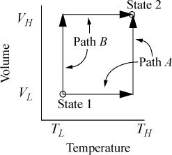
Figure 8.1. Comparison of two alternate paths for calculation of a change of state.
Path A:
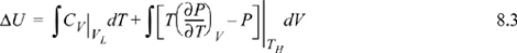
or Path B:
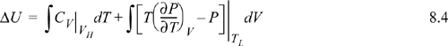
We have previously shown, in Example 7.6 on page 269, that CV depends on volume for a real fluid. Therefore, even though we could insert the equation of state for the integrand of the second integral, we must also estimate CV by the equation of state for at least one of the volumes, using the results of Example 7.6. Not only is this tedious, but estimates of CV by equations of state tend to be less reliable than estimates of other properties.
To avoid this calculation, we devise an equivalent pathway of three stages. First, imagine if we had a magic wand to turn our fluid into an ideal gas. Second, the ideal gas state change calculations would be pretty easy. Third, at the final state we could turn our fluid back into a real fluid. Departure functions represent the effect of the magic wand to exchange the real fluid with an ideal gas. Being careful with signs of the terms, we may combine the calculations for the desired result:

The calculation can be generalized to any fundamental property from the set {U,H,A,G,S}, using the variable M to denote the property

![]() Departure functions permit us to use the ideal gas calculations that are easy, and incorporate a departure property value for the initial and final states.
Departure functions permit us to use the ideal gas calculations that are easy, and incorporate a departure property value for the initial and final states.
The steps can be seen graphically in Fig. 8.2. Note the dashed lines in the figure represent the calculations from our “magic wand” effect of turning on/off the nonidealities.
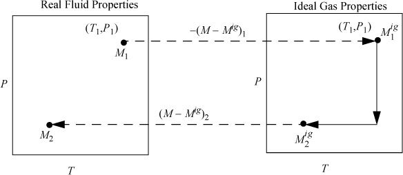
Figure 8.2. Illustration of calculation of state changes for a generic property M using departure functions where M is U, H, S, G, or A.
Note how all the ideal gas terms in Eqns. 8.5 and 8.6 cancel to yield the desired property difference. A common mistake is to get the sign wrong on one of the terms in these equations. Make sure that you have the terms in the right order by checking for cancellation of the ideal gas terms. The advantage of this pathway is that all temperature calculations are done in the ideal gas state where:

and the ideal gas heat capacities are pressure- (and volume-) independent (see Example 6.9 on page 242).
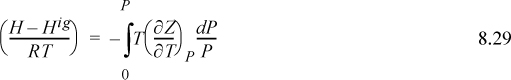
To derive the formulas to be used in calculating the values of enthalpy, internal energy, and entropy for real fluids, we must apply our fundamental property relations once and our Maxwell’s relations once.
8.2. Internal Energy Departure Function
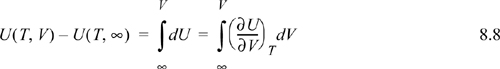
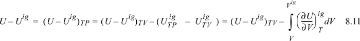
Fig. 8.3 schematically compares a real gas isotherm and an ideal gas isotherm at identical temperatures. At a given {T,P} the volume of the real fluid is V, and the ideal gas volume is Vig = RT/P. Similarly, the ideal gas pressure is not equal to the true pressure when we specify {T,V}. Note that we may characterize the departure from ideal gas behavior in two ways: 1) at the same {T,V}; or 2) at the same {T,P}. We will find it convenient to use both concepts, but we need nomenclature to distinguish between the two departure characterizations. When we refer to the departure of the real fluid property and the same ideal gas property at the same {T,P}, we call it simply the departure function, and use the notation U – Uig. When we compare the departure at the same {T,V} we call it the departure function at fixed T,V, and designate it as (U – Uig)TV.1
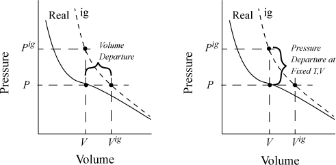
Figure 8.3. Comparison of real fluid and ideal gas isotherms at the same temperature, demonstrating the departure function, and the departure function at fixed T,V.
To calculate the change in internal energy along an isotherm for the real fluid, we write:
![]() The departure for property M is at fixed T and, P and is given by (M–Mig). The departure at fixed T,V is also useful (particularly in Chapter 15) and is denoted by (M–Mig)TV.
The departure for property M is at fixed T and, P and is given by (M–Mig). The departure at fixed T,V is also useful (particularly in Chapter 15) and is denoted by (M–Mig)TV.
For an ideal gas:
Since the real fluid approaches the ideal gas at infinite volume, we may take the difference in these two equations to find the departure function at fixed T,V,
where (U – Uig)T, V = ∞ drops out because the real fluid energy approaches the ideal gas at infinite volume (low pressure). We have obtained a calculation with the real fluid in our desired state (T,P,V); however, we are referencing an ideal gas at the same volume rather than the same pressure. To see the difference, consider methane at 250 K, 10 MPa, and 139 cm3/mole. The volume of the ideal gas should be Vig = 8.314·250/10 = 208 cm3/mole. To obtain the departure function denoted by (U – Uig) (which is referenced to an ideal gas at the same pressure), we must add a correction to change the ideal gas state to match the pressure rather than the volume. Note in Fig. 8.3 that the real state is the same for both departure functions—the difference between the two departure functions has to do with the volume used for the ideal gas part of the calculation. The result is
We have already solved for (∂Uig/∂V)T (see Example 6.6 on page 238), and found that it is equal to zero. We are fortunate in this case because the internal energy of an ideal gas does not depend on the volume. When it comes to properties involving entropy, however, the dependency on volume requires careful analysis. Then the systematic treatment developed above is quite valuable.

Making these substitutions, we have
If we transform the integral to density, the resultant expression is easier to integrate for a cubic equation of state. Recognizing dV = –dρ/ρ2, and as V → ∞, ρ → 0, thus,
The above equation applies the chain rule in a way that may not be obvious at first:

We now have a compact equation to apply to any equation of state. Knowing Z = Z(T, ρ), (e.g., Eqn. 7.15, the Peng-Robinson model), we simply differentiate once, cancel some terms, and integrate. This a perfect sample application of the multivariable calculus that should be familiar at this stage in the curriculum. More importantly, we have developed a systematic approach to solving for any departure function. The steps for a system where Z = Z(T, ρ) are as follows.
1. Write the derivative of the property with respect to volume at constant T. Convert to derivatives of measurable properties using methods from Chapter 6.
2. Write the difference between the derivative real fluid and the derivative ideal gas.
3. Insert integral over dV and limits from infinite volume (where the real fluid and the ideal gas are the same) to the system volume V.
4. Add the necessary correction integral for the ideal gas from V to Vig. (This will be more obvious for entropy.)
5. Transform derivatives to derivatives of Z. Evaluate the derivatives symbolically using the equation of state and integrate analytically.
6. Rearrange in terms of density and compressibility factor to make it more compact.
Some of these steps could have been omitted for the internal energy, because (∂Uig/∂V)T = 0. Steps 1 through 4 are slightly different when Z = Z(T, P) such as with the truncated virial EOS. To see the importance of all the steps, consider the entropy departure function.
Example 8.1. Internal energy departure from the van der Waals equation
Derive the internal energy departure function for the van der Waals equation. Suppose methane is compressed from 200 K and 0.1 MPa to 220 K and 60 MPa. Which is the larger contribution in magnitude to ΔU, the ideal gas contribution or the departure function? Use CP from the back flap and ignore temperature dependence.
Solution
For methane, a = 230030 J-cm3/mol2 and b = 43.07 cm3/mol were calculated by the critical point criteria in Example 7.7 on page 271. Deriving the departure function, –T(dZ/dT)ρ = –aρ/RT, because the repulsive part is constant with respect to T. Substituting,
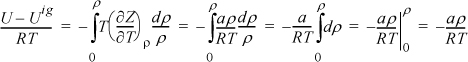
Because Tr > 1 there is only one real root. A quick but crude computation of ρ is to rearrange as Zbρ = bP/RT = bρ/(1 – bρ) – (a/bRT)(bρ)2.
At state 2, 220 K and 60 MPa,
60·43.07/(8.314·220) = bρ/(1 – bρ) – 230030/(43.07·8.314·220)(bρ)2.
Taking an initial guess of bρ = 0.99 and solving iteratively gives bρ = 0.7546, so
(U2 – U2ig)/RT = –230030·0.7546/(43.07·8.314·220) = –2.203.
At state 1, 200 K and 0.1 MPa,
0.1·43.07/(8.314·200) = bρ/(1 – bρ) – 230030/(43.07·8.314·200)(bρ)2.
Taking an initial guess of bρ = 0.99 and solving iteratively gives bρ = 0.00290, so
(U1 – U1ig)/RT = –230030·0.00290/(43.07·8.314·200) = –0.00931.

ΔU = –2.203(8.314)220 + (4.3 – 1)·8.314(220 – 200) + 0.00931(8.314)200 = –4030 + 549 + 15 = –3466 J/mol. The ideal gas part (549) is 14% as large in magnitude as the State 2 departure function (–4030) for this calculation. Clearly, State 2 is not an ideal gas.
Note that we do not need to repeat the integral for every new problem. For the van der Waals equation, the formula (U–Uig)/(RT) = –(aρ)/(RT) may readily be used whenever the van der Waals fluid density is known for a given temperature.
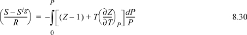
8.3. Entropy Departure Function
To calculate the entropy departure, adapt Eqn. 8.11,
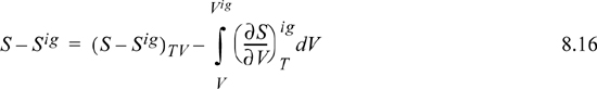
Inserting the integral for the departure at fixed {T, V}, we have (using a Maxwell relation),
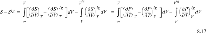
Since ![]() , we may readily integrate the ideal gas integral (note that this is not zero whereas the analogous equation for energy was zero):
, we may readily integrate the ideal gas integral (note that this is not zero whereas the analogous equation for energy was zero):
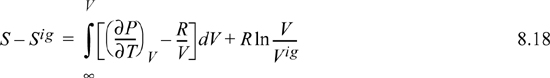
Recognizing Vig = RT/P, V/Vig = PV/RT = Z,
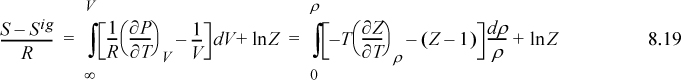
where Eqn. 8.15 has been applied to the relation for the partial derivative of P.
Note the ln(Z) term on the end of this equation. It arises from the change in ideal gas ![]() represented by the integral in Eqn. 8.16. Changes in states like this may seem pedantic and arcane, but they turn out to be subtle details that often make a big difference numerically. In Example 7.4 on page 266, we determined vapor and liquid roots for Z. The vapor root was close to unity, so ln(Z) would make little difference in that case. For the liquid root, however, Z = 0.016, and ln(Z) makes a substantial difference. These arcane details surrounding the subject of state specification are the thermodynamicist’s curse.
represented by the integral in Eqn. 8.16. Changes in states like this may seem pedantic and arcane, but they turn out to be subtle details that often make a big difference numerically. In Example 7.4 on page 266, we determined vapor and liquid roots for Z. The vapor root was close to unity, so ln(Z) would make little difference in that case. For the liquid root, however, Z = 0.016, and ln(Z) makes a substantial difference. These arcane details surrounding the subject of state specification are the thermodynamicist’s curse.
8.4. Other Departure Functions
The remainder of the departure functions may be derived from the first two and the definitions,

![]() The departures for U and S are the building blocks from which the other departures can be written by combining the relations derived in the previous sections.
The departures for U and S are the building blocks from which the other departures can be written by combining the relations derived in the previous sections.
where we have used PVig = RT for the ideal gas in the enthalpy departure. Using H – Hig just derived,

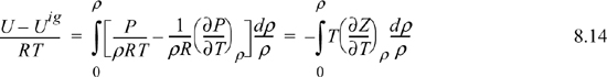
8.5. Summary of Density-Dependent Formulas
Formulas for departures at fixed T,P are listed below. These formulas are useful for an equation of state written most simply as Z = f(T,ρ) such as cubic EOSs. For treating cases where an equation of state is written most simply as Z = f (T,P) such as the truncated virial EOS, see Section 8.6.


Useful formulas at fixed T,V include:


8.6. Pressure-Dependent Formulas
Occasionally, our equation of state is difficult to integrate to obtain departure functions using the formulas from Section 8.5. This is because the equation of state is more easily arranged and integrated in the form Z = f (T,P), such as the truncated virial EOS. For treating cases where an equation of state is written most simply as Z = f(T,ρ) such as a cubic EOS, see Section 8.5. We adapt the procedures given earlier in Section 8.2.
1. Write the derivative of the property with respect to pressure at constant T. Convert to derivatives of measurable properties using methods from Chapter 6.
2. Write the difference between the derivative real fluid and the derivative ideal gas.
3. Insert integral over dP and limits from P = 0 (where the real fluid and the ideal gas are the same) to the system pressure P.
4. Transform derivatives to derivatives of Z. Evaluate the derivatives symbolically using the equation of state and integrate analytically.
5. Rearrange in terms of density and compressibility factor to make it more compact.
We omit derivations and leave them as a homework problem. The two most important departure functions at fixed T,P are
The other departure functions can be derived from these using Eqns. 8.20 and 8.21. Note the mathematical similarity between P in the pressure-dependent formulas and ρ in the density-dependent formulas.
8.7. Implementation of Departure Formulas
The tasks that remain are to select a particular equation of state, take the appropriate derivatives, make the substitutions, develop compact expressions, and add up the change in properties. The good news is that many years of engineering research have yielded several preferred equations of state (see Appendix D) which can be applied generally to any application with a reasonable degree of accuracy. For the purposes of the text, we use the Peng-Robinson equation or virial equation to illustrate the principles of calculating properties. However, many applications require higher accuracy; new equations of state are being developed all the time. This means that it is necessary for each student to know how to adapt the departure function method to new situations as they come along.
The following example illustrates the procedure with an equation of state that is sufficiently simple that it can be applied with either the density-dependent formulas or the pressure-dependent formulas. Although the intermediate steps are a little different, the final answer is the same, of course.
Example 8.2. Real entropy in a combustion engine
A properly operating internal combustion engine requires a spark plug. The cycle involves adiabatically compressing the fuel-air mixture and then introducing the spark. Assume that the fuel-air mixture in an engine enters the cylinder at 0.08 MPa and 20°C and is adiabatically and reversibly compressed in the closed cylinder until its volume is 1/7 the initial volume. Assuming that no ignition has occurred at this point, determine the final T and P, as well as the work needed to compress each mole of air-fuel mixture. You may assume that ![]() for the mixture is 32 J/mole-K (independent of T), and that the gas obeys the equation of state,
for the mixture is 32 J/mole-K (independent of T), and that the gas obeys the equation of state,
PV = RT + aP
where a is a constant with value a = 187 cm3/mole. Do not assume that CV is independent of ρ. Solve using density integrals.
Leave a Reply