Suppose that in a spreadsheet the following formula is entered into cell B1:

Since cell reference B1 is in the formula of the same cell, this is called a “circular reference.” Normally, Excel will complain about this. However, if the Enable Iterative Calculations (see File/Options/Formulas) box is checked, Excel will immediately do the following:

1. It will automatically use an initial guess of zero (there is no control over this).

2. It will iterate up to 100 times or until successive values are within 0.001 (these values can be changed).

3. The final result will be the answer (hopefully).

In-cell iteration is not to be encouraged when robustness is a goal. It often fails to find a solution.

EXERCISES

Exercise 1.1: For the following functions, graph the function and then use Goal Seek to find the root(s).

a. f(x) = x − x^1/3 − 2

b. f(x) = xtanx − 1

c. f(x) = x⁴ − e^x + 1

d. f(x) = x²e^x − 1

Exercise 1.2: Find the roots of the functions given in Exercise 1.1 using the bisection method. Use the graph of each function to choose points that bracket the root of interest.

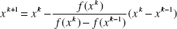
Exercise 1.3: Set up a spreadsheet that implements the secant method and then solve each of the problems from Exercise 1.1. Use the graph of each function to select an initial guess. Recall the iteration formula for the secant method:

Hint: Set up the first row of the spreadsheet for your problem with headings such as the following:

Put the formula for the function under the headings f(xk-1) and f(xk). In the cell under xk+1, put the secant method iteration formula. In the second row, replace the previous xk-1 with xk and then xk with xk+1. Now copy the two formulas down one row. At this point, one iteration of the secant method is displayed. To see more iterations, just copy the second row down for as many iterations as desired. If too many iterations are copied and the function difference (the denominator of the iteration formula) becomes exactly zero, a “divide by zero” error will appear.

Exercise 1.4: Use Goal Seek to find root(s) of the following functions. Plot the functions first to obtain an approximation of a desired root.

a. f(x) = x³ – 17x + 12 = 0

b. J₁(x) = 0 J₁ is the Bessel function of the first kind of order 1. It can be computed in Excel using the BESSELJ()function. This function has an infinite number of roots; find the root between 2 and 5.

c. Solve for the molar volume of a gas at 400 K and 1200 kPa using the van der Waals equation of state. The critical temperature and pressure are 500 K and 80 atm, respectively. Use the ideal gas solution for your initial guess.

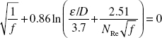
d. Solve the Colebrook equation for the Darcy friction factor, f, for a Reynolds number (N_Re) of 10⁵ and a roughness factor, ε/D, of 10⁻⁴ (this equation holds for Reynolds numbers > 4000):

e. Repeat part d using the same roughness factor, but for a range of Reynolds numbers from 5000 to 30,000 (pick a reasonable increment). Plot the results (friction factor versus Reynolds number). Automate Goal Seek for this.

Exercise 1.5: Use the secant method as described in Exercise 1.3 to find the root(s) of the functions given in Exercise 1.4. Carefully choose the two initial guesses so that the function values have opposite signs. The roots found may or may not correspond to those found using Goal Seek in Exercise 1.3—it depends on the initial guesses.

Exercise 1.6: Solve the problems of Exercise 1.1 using the Newton method.

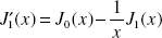
Exercise 1.7: Repeat Exercise 1.4 parts a and b using the Newton method. The derivative of J₁(x) is given by

Exercise 1.8: Repeat Exercise 1.4 using the bisection method.

Exercise 1.9: An additional method for solving single nonlinear equation is the “Regula–Falsi” or method of “false position.” Like the bisection method, the false position method starts with two points a₀ and b₀ such that f(a₀) and f(b₀) are of opposite signs, which implies that the function f has a root in the interval [a₀, b₀]. The Regula–Falsi method proceeds by producing a sequence of shrinking intervals [a_k, b_k] that always contain a root of f.

    At iteration number k, the value

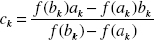
is computed. As explained below, c_k is the root of the secant line through (a_k, f(a_k)) and (b_k, f(b_k)). If f(a_k) and f(c_k) have the same sign, then set a_k+1 = c_k and b_k+1 = b_k; otherwise set a_k+1 = a_k and b_k+1 = c_k. This process is repeated until the root is approximated sufficiently well.

The above formula is also used in the secant method, but the secant method always retains the last two computed points, while the false position method retains two points that bracket a root. On the other hand, the only difference between the false position method and the bisection method is that the latter uses c_k = (a_k + b_k)/2.

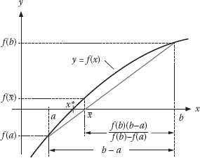
FIGURE 1.7 Regula–Falsi method.

A schematic description of the Regula–Falsi method is shown in Figure 1.7.

Repeat either Exercise 1.1 or 1.4 using the method of false position.

Exercise 1.10: Refer to the diagram and data of Example 1.7. The dew point of a vapor is the temperature at a given pressure at which the first drop of liquid is formed. Thus, at the dew point, the ratio of vapor to feed (V/F) is essentially one. Conversely, the bubble point of a liquid is the temperature at a given pressure at which the first bubble of vapor is formed and at this condition V/F = 0.

Assume, as in Example 1.7, an ideal mixture (where Raoult’s law applies). Also, assume the same mixture and data as shown in Figure 1.4.

a. At the dew point, V/F = 1 [there is an infinitesimal amount of liquid, but it does exist and has a mole fraction for each component (x_i); however, since there is only an infinitesimal amount of liquid, V = F and y_i = z_i]. Applying the fact that the sum of x_i = 1, the following equation results:

Since k_j are functions of temperature, this nonlinear equation can be solved for the temperature (dew point).

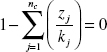
b. At the bubble point, V/F = 0 (L/F = 1) and x_i = z_i, and if that fact that the sum of y_i = 1 is applied, the following equation results:

This nonlinear equation can be solved for the temperature (bubble point).

The specific assignment is as follows.

1. Prepare an Excel spreadsheet that calculates for a mixture the bubble point at pressures of 15, 16, …, 25 atm and produces a plot of the bubble point versus pressure with suitable annotations and title. Use Goal Seek to solve the single nonlinear equation at each pressure. Data for the system are given in Figure 1.4.