As a state property, the molar (or specific) volume can be determined once as a function of pressure and temperature, and tabulated for future use. Tabulations have been compiled for a large number of pure fluids. In very common use are the steam tables, which contain tabulations of the properties of water. Steam is a basic utility in chemical plants as a heat transfer fluid for cooling or heating, as well as for power generation (pressurized steam), and its properties are needed in many routine calculations. Thermodynamic tables for water are published by the American Society of Mechanical Engineers (ASME) and are available in various forms, printed and electronic. A copy is included in the appendix. We will use them not only because water is involved in many industrial processes but also as a demonstration of how to work with tabulated values in general.
Note
Interpolations
When working with tabulated values it is necessary to perform interpolations if the desired conditions lie between entries in the table. Suppose that a table contains the values of a function f (x) at x = x1 and x = x2 and we wish to obtain the value of f at an intermediate point x such that x1 < x < x2, we assume a linear relationship between f and x and write

where f1, f2 are the values of the function at points x1, x2, respectively. The procedure is shown graphically in Figure 2-5a. If the value of x is outside the interval (x1, x2), the same formula may be used and this calculation is called an extrapolation. Extrapolations should be avoided because they can be subject to large error. They may be used if the desired value is beyond the last tabulated entry, however, one cannot be certain about the accuracy of the result.
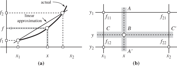
Figure 2-5: Linear interpolation: (a) simple interpolation; (b) double interpolation.
In thermodynamics we are usually dealing with functions of two variables, for example, f (x, y). If point (x, y) is such that the value y is found in the table but the value of x falls between tabulated values, the above equation may be used to interpolate with respect to x. If both x and y fall between tabulated entries, a double interpolation is necessary. The procedure involves three simple interpolations, and can be outlined as follows (Figure 2-5b): first interpolate between the tabulated values at (x1, y1) and (x1, y2) to obtain the value of f at point C; do the same between points (x2, y1) and (x2, y2) to obtain f at point C′. Finally, interpolate between C and C′ to obtain the value at the desired point B. Alternatively, interpolate to obtain points A and A′ followed by interpolation between A and A′ to obtain B—the result is the same. These steps can be combined into a single equation which takes the form:

with

Here, the notation fij refers to f(xi, yj). If both a and b are between 0 and 1, this calculation is indeed an interpolation and produces a result that is surrounded by the four tabulated values used in the calculation. This equation can be used for extrapolations outside these four values provided the distance is not large.
Use the steam tables to determine the specific volume of water at 1.25 bar, 185 °C.
Solution From the superheated steam tables we find the following values for the specific volume (in m3/kg):
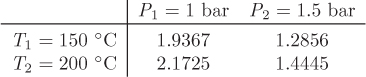
In this problem, pressure (1.25 bar) and temperature (185 °C) both lie between the tabulated values. Therefore, a double interpolation is required. We do the calculation first by successive interpolations, then by applying equation (2.14) for double interpolations.
Method 1—successive interpolations: We first obtain the volume at P = 1.25 bar, T1 = 150 °C by interpolation between the values listed in the first row of the above data:

This amounts to obtaining the volume at point C of Figure 2-5. Next, we obtain the volume at P = 1.25 bar, T1 = 200 °C by interpolation between the values listed in the second row:

This amounts to calculating the volume at point C′. Finally, we interpolate between V1 (point C) and V2 (C′) to obtain the volume at 1.25 bar, 185 °C:

The result corresponds to point B in Figure 2-5.
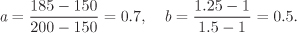
Method II—double interpolation: To apply the double-interpolation formula, we take x to be temperature and y to be pressure, and fxy to be the specific volume at temperature x and pressure y. The factors a and b are calculated from eq. (2.15):
The interpolated volume is
V = (1 − 0.7)(1 − 0.5)(1.9367) + (0.5)(1 − 0.7)(1.2856)+ (0.7)(1 − 0.5)(2.1725) + (0.7)(0.5)(1.4445) = 1.7493 m3/kg.
Both methods give the same answer, as they should.
Example 2.5: Locating the State in the Steam Tables
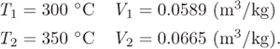
A 12m3 pressurized vessel contains 200 kg of steam at 40 bar. What is the temperature?
Solution The specific volume of the steam in the tank is
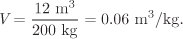
We know two intensive properties, pressure and specific volume; the state, therefore, is fully specified. We must locate a point in the steam tables with P = 40 bar, V = 0.06 m3/kg.
From the entries at 40 bar we obtain the following data:
Interpolating for temperature at V = 0.06 m3/kg we have

Therefore, the temperature in the tank is 307.2 °C.
An additional 170 kg of steam is added to the tank of the previous example. If the final pressure is 50 bar, determine the temperature and phase of the contents of the tank.
Solution The new specific volume is
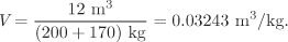
This volume lies between the volume of the saturated liquid and saturated vapor at 50 bar:
P = 50 bar T = 263.94 °C: VL = 0.0012864 m3/kg, VV = 0.039446 m3/kg.
The state, therefore, is wet steam at 50 bar, 263.94 °C. To determine the mass fractions of each phase we use the lever rule in eq. (2.10):
Therefore, the quality of the steam in the tank is 81.6%.
2.3 Compressibility Factor and the ZP Graph
The compressibility factor, Z, is defined as the ratio
where V is the molar volume, P is pressure, and T is absolute temperature. It is a dimensionless quantity and a state function. In the ideal-gas state, Vig = RT/P, and the compressibility factor is unity:

More precisely, this is the limiting value of the compressibility factor of any real gas when pressure is reduced to zero under constant temperature:

This result states that the compressibility factor along a line of constant temperature goes to 1 as P is reduced to zero. In other words, on a graph of Z versus pressure, all isotherms at zero pressure must meet at Z = 1.
The compressibility factor represents an alternative way of presenting molar volume, since the molar volume can be obtained easily if the compressibility factor is known at a given pressure and temperature:

Mathematically, the equation of state can be represented as either a relationship between P, V, and T, or between Z, P, and T. The latter relationship is quite useful in presenting the volumetric behavior of fluids. Its graphical representation is given on the ZP graph, whose general form is shown in Figure 2-6. Here again we have the vapor-liquid boundary in the form of bell-shaped curve that is now seated on the vertical axis. The vapor region is at the top, the liquid at the bottom. Generally, compressibility factors in the liquid phase are smaller than those in the vapor phase because the molar volume of the liquid is small. All isotherms meet at P = 0, Z = 1, as anticipated on the basis of eq. (2.18). This point of convergence represents the ideal-gas state. The ZP graph illustrates the path to the ideal-gas state: it is approached by following an isotherm to zero pressure. Since all isotherms converge to this point, the ideal-gas state can be reached from any initial state. We can now see why there is no such a thing as an ideal-gas state: if such a gas existed, its ZP graph would consist of a single horizontal line at Z = 1, which would represent all isotherms. No substance exists that exhibits such behavior.
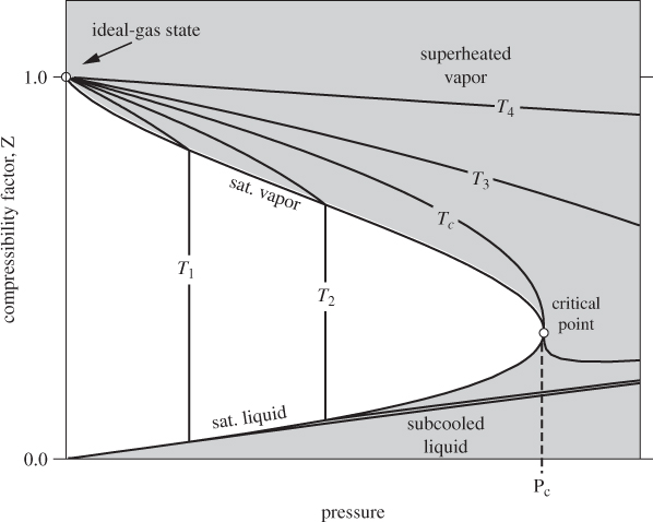
Figure 2-6: The ZP graph of pure fluid.
Although the mathematical definition places the ideal-gas state at a single point (P = 0, Z = 1), from a practical point of view we will consider a gas to be in the ideal-gas state if the compressibility factor is sufficiently close to 1. For calculations that do not require high accuracy we will assume a gas to be in the ideal-gas state if the compressibility factor is within ±5% of the theoretical value of 1. The pressure range over which this approximation is valid varies with temperature.
With reference to Figure 2-6, the isotherm at T4 remains closer to 1 over a wider interval of pressures, compared to the isotherm at T1, which has a larger negative slope and decreases faster. In general, to determine whether a gas at given pressure and temperature can be treated as ideal we must check with a ZP graph. We will return to this question in the next section.
2.4 Corresponding States
It is found experimentally that the ZP graphs of different fluids look very similar to each other as if they are scaled versions of a single, universal, graph. This underlying graph is revealed if pressure and temperature are rescaled by appropriate factors. We introduce a set of reduced (dimensionless) variables by scaling pressure and temperature with the corresponding values at the critical point:

Using the reduced coordinates it is possible to combine ZP data for several compounds on the same graph. Figure 2-7 shows the resulting graph for selected molecules. The remarkable feature of this graph is that the compressibility factor of the six compounds shown on this figure agree with each other quite well. Even though the dependence of the compressibility factor on temperature and pressure is different for each fluid, they all seem to arise from the same reduced function. This observation gives rise to the correlation of corresponding states, which is expressed as follows:
At the same reduced temperature and pressure, fluids have approximately the same compressibility factor.
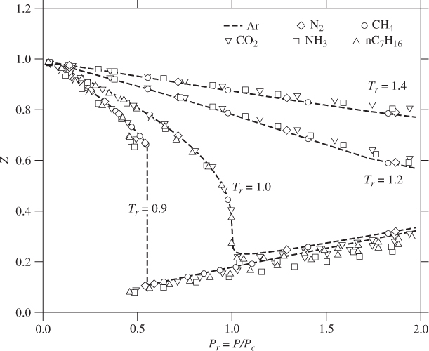
Figure 2-7: The compressibility factor of selected molecules as a function of reduced pressure and temperature. Data compiled from E. W. Lemmon, M. O. McLinden and D. G. Friend, “Thermophysical Properties of Fluid Systems.” In NIST Chemistry WebBook, NIST Standard Reference Database No. 69, eds. P. J. Linstrom and W. G. Mallard, National Institute of Standards and Technology, Gaithersburg MD, 20899, http://webbook.nist.gov (retrieved December 11, 2010).
We express this mathematically by writing,

The practical implication is important: to the extent that eq. (2.20) is obeyed, the compressibility factor of any fluid can be described by a universal equation that is a function of reduced temperature and reduced pressure. Figure 2-7 is a graphical representation of this equation. Accordingly, the compressibility factor of a fluid can be determined at any pressure and temperature using just two parameters, the critical temperature and critical pressure.
The correlation of corresponding states is not an exact physical law and is not obeyed to the same degree of accuracy by all fluids. Although the agreement in Figure 2-7 between different fluids is impressive, it is not exact. The spread of the data points in Figure 2-7 is not due to experimental error (the values have been calculated from validated models) but reflect systematic deviations. These are more clearly seen near the saturation curve and in the liquid region. The correlation arises from similarities in the intermolecular potential. In general, agreement is very good in the gas phase, where interactions are unimportant. In the liquid region, interactions are important and the individual chemical character of molecules becomes more apparent. Even so, nonpolar molecules that are nearly spherical in shape (e.g., Ar, CH4) agree remarkably well. Polar molecules or molecules with more complex structures (e.g., normal heptane) show the largest deviations because their interactions are more complex and dissimilar. Molecules like water, which is both polar and associates strongly via hydrogen bonding, exhibit even more deviations from this correlation. The principle of corresponding states should be treated as a working hypothesis that can provide useful but not always highly accurate estimates of the compressibility factor.
Acentric Factor and the Pitzer Method
Eq. (2.20) is a two-parameter correlation because it requires two physical properties, critical temperature and critical pressure. To improve the predictive power of the principle of corresponding state while retaining its simplicity, a third parameter is introduced, the acentric factor. It is a dimensionless parameter that is defined according to the equation,

where ![]() is the reduced saturation pressure of the fluid at reduced temperature Tr = 0.7. It is a characteristic property of the fluid and is found in tables, usually along with the critical properties of the fluid. It was introduced by Pitzer as a measure of the sphericity of the molecule. More generally, it should be understood as a combined measure of the shape and polarity. Symmetric nonpolar molecules, such as Ar, have ω = 0. These are called simple fluids and are found to obey the two-parameter correlation of corresponding states quite well. Nonspherical or polar molecules have a larger acentric factor. For most fluids the acentric factor is positive and in the range 0 to 0.4, although small negative values of ω are also possible.
is the reduced saturation pressure of the fluid at reduced temperature Tr = 0.7. It is a characteristic property of the fluid and is found in tables, usually along with the critical properties of the fluid. It was introduced by Pitzer as a measure of the sphericity of the molecule. More generally, it should be understood as a combined measure of the shape and polarity. Symmetric nonpolar molecules, such as Ar, have ω = 0. These are called simple fluids and are found to obey the two-parameter correlation of corresponding states quite well. Nonspherical or polar molecules have a larger acentric factor. For most fluids the acentric factor is positive and in the range 0 to 0.4, although small negative values of ω are also possible.
In the Pitzer method, the compressibility factor is expressed in the form:

where Z(0) and Z(1) are universal functions that depend on Tr and Pr. Function Z(0) represents the compressibility factor of simple fluids (ω = 0) and Z(1) represents a correction that is proportional to the acentric factor. The two functions Z(0) and Z(1) may be calculated once and tabulated against reduced pressure and temperature for future use. The resulting tables and charts are called generalized because they are not limited to a specific molecule.
Various methodologies have been developed for the calculation of the functions in eq. (2.22), but the most widely used is that of Lee and Kesler.5 The Lee-Kesler result for Z(0) is plotted in Figure 2-8. Recall that this term represents the compressibility factor of a simple fluid, therefore, it has the familiar appearance of the ZP graph. Figure 2-9 shows the same graph in semi-logarithmic scales that cover an expanded range of pressures. The Z(1) is shown in Figure 2-10. The correction factor is zero in the vicinity of the ideal-gas state. It increases in absolute value with increasing pressure and it may take positive or negative values. The sharp changes in subcritical temperatures correspond to a shift from the vapor branch to the liquid branch of the isotherm. The vapor/liquid transitions in Figures 2-8, 2-9, and 2-10 apply only to simple fluids (ω = 0). For nonsimple fluids the phase boundary also depends on the acentric factor ω and is generally shifted to lower reduced pressure compared to simple fluids.6
5. B. I. Lee and M. G. Kesler. A generalized thermodynamic correlation based on three-parameter corresponding states. AIChE J., 21(3):510, 527 1975. doi: 10.1002/aic.690210313.
6. The determination of the precise location of the phase boundary is discussed in Chapter 7.
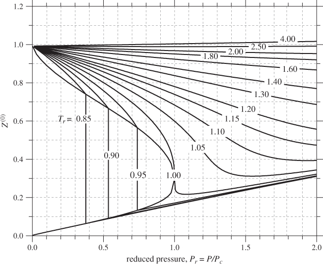
Figure 2-8: Generalized graph of Z(0) based on the Lee-Kesler method.
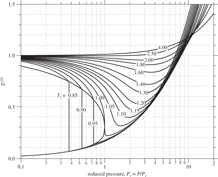
Figure 2-9: Generalized graph of Z(0) based on the Lee-Kesler calculation (extended range of pressures).
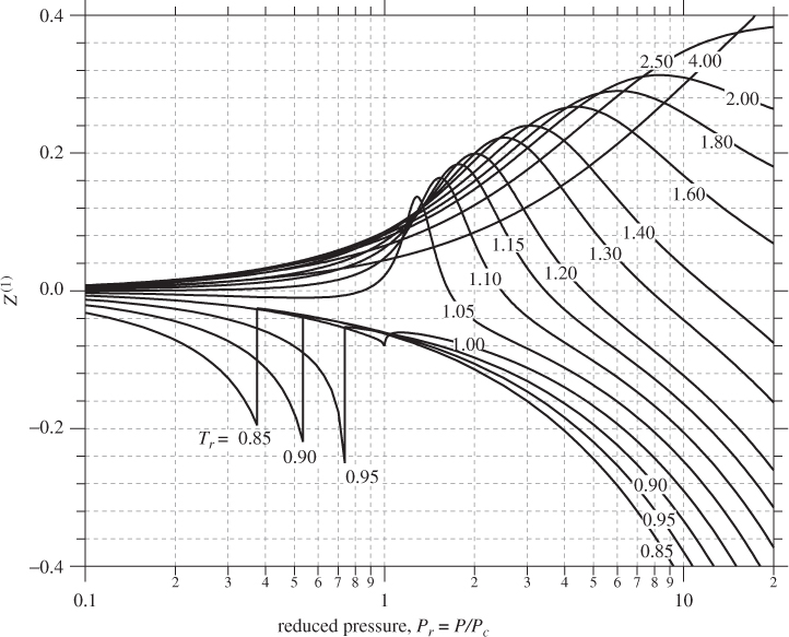
Figure 2-10: Generalized graph of Z(1) based on the Lee-Kesler calculation.
Leave a Reply