All macroscopic behavior of matter is the result of phenomena that take place at the microscopic level and arise from force interactions among molecules. Molecules exert a variety of forces: direct electrostatic forces between ions or permanent dipoles; induction forces between a permanent dipole and an induced dipole; forces of attraction between nonpolar molecules, known as van der Waals (or dispersion) forces; other specific chemical forces such as hydrogen bonding. The type of interaction (attraction or repulsion) and the strength of the force that develops between two molecules depends on the distance between them. At far distances the force is zero. When the distance is of the order of several Å, the force is generally attractive. At shorter distances, short enough for the electron clouds of the individual atoms to begin to overlap, the interaction becomes very strongly repulsive. It is this strong repulsion that prevents two atoms from occupying the same point in space and makes them appear as if they possess a solid core. It is also the reason that the density of solids and liquids is very nearly independent of pressure: molecules are so close to each other that adding pressure by any normal amounts (say 10s of atmospheres) is insufficient to overcome repulsion and cause atoms to pack much closer.
Intermolecular Potential
The force between two molecules is a function of the distance between them. This force is quantified by intermolecular potential energy, Φ(r), or simply intermolecular potential, which is defined as the work required to bring two molecules from infinite distance to distance r. Figure 1-3 shows the approximate intermolecular potential for CO2. Carbon dioxide is a linear molecule and its potential depends not only on the distance between the molecules but also on their relative orientation. This angular dependence has been averaged out for simplicity. To interpret Figure 1-3, we recall from mechanics that force is equal to the negative derivative of the potential with respect to distance:
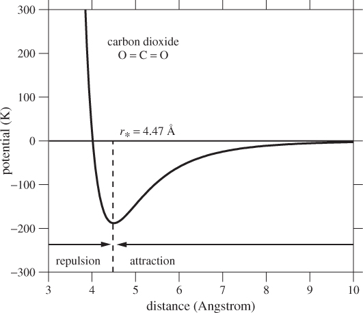
Figure 1-3: Approximate interaction potential between two CO2 molecules as a function of their separation distance. The potential is given in kelvin; to convert to joule multiply by the Boltzmann constant, kB = 1.38 × 10⁻²³ J/K. The arrows show the direction of the force on the test molecule in the regions to the left and to the right of r*.
That is, the magnitude of the force is equal to the slope of the potential with a negative sign that indicates that the force vector points in the direction in which the potential decreases. To visualize the force, we place one molecule at the origin and a test molecule at distance r. The magnitude of the force on the test molecule is equal to the derivative of the potential at that point (the force on the first molecule is equal in magnitude and opposite in direction). If the direction of force is towards the origin, the force is attractive, otherwise it is repulsive. The potential in Figure 1-3 has a minimum at separation distance r* = 4.47 Å. In the region r > r* the slope is positive and the force is attractive. The attraction is weaker at longer distances and for r larger than about 9 Å the potential is practically flat and the force is zero. In the region r < r* the potential is repulsive and its steep slope indicates a very strong force that arises from the repulsive interaction of the electrons surrounding the molecules. Since the molecules cannot be pushed much closer than about r ≈ r*, we may regard the distance r* to be the effective diameter of the molecule.1 Of course, even simple molecules like argon are not solid spheres; therefore, the notion of a molecular diameter should not be taken literally.
1. The closest center-to-center distance we can bring two solid spheres is equal to the sum of their radii. For equal spheres, this distance is equal to their diameter.
The details of the potential vary among different molecules but the general features are always the same: Interaction is strongly repulsive at very short distance, weakly attractive at distance of the order of several Å, and zero at much larger distances. These features help to explain many aspects of the macroscopic behavior of matter.
Temperature and Pressure
In the classical view of molecular phenomena, molecules are small material objects that move according to Newton’s laws of motion, under the action of forces they exert on each other through the potential interaction. Molecules that collide with the container walls are reflected back, and the force of this collision gives rise to pressure. Molecules also collide among themselves,2 and during these collisions they exchange kinetic energy. In a thermally equilibrated system, a molecule has different energies at different times, but the distribution of energies is overall stationary and the same for all molecules. Temperature is a parameter that characterizes the distribution of energies inside a system that is in equilibrium with its surroundings. With increasing temperature, the energy content of matter increases. Temperature, therefore, can be treated as a measure of the amount of energy stored inside matter.
2. Molecular collisions do not require solid contact as macroscopic objects do. If two molecules come close enough in distance, the steepness of the potential produces a strong repulsive force that causes their trajectories to deflect.
Note
Maxwell-Boltzmann Distribution
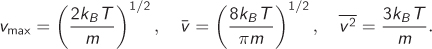
The distribution of molecular velocities in equilibrium is given by the Maxwell-Boltzmann equation:

where m is the mass of the molecule, v is the magnitude of the velocity, T is absolute temperature, and kB is the Boltzmann constant. The fraction of molecules with velocities between any two values v1 to v2 is equal to the area under the curve between the two velocities (the total area under the curve is 1). The velocity vmax that corresponds to the maximum of the distribution, the mean velocity s![]() , and the mean of the square of the velocity are all given in terms of temperature:
, and the mean of the square of the velocity are all given in terms of temperature:
The Maxwell-Boltzmann distribution is a result of remarkable generality: it is independent of pressure and applies to any material, regardless of composition or phase. Figure 1-4 shows this distribution for water at three temperatures. At the triple point, the solid, liquid, and vapor, all have the same distribution of velocities.
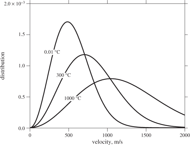
Figure 1-4: Maxwell-Boltzmann distribution of molecular velocities in water.
Phase Transitions
The minimum of the potential represents a stable equilibrium point. At this distance, the force between two molecules is zero and any small deviations to the left or to the right produce a force that points back to the minimum. A pair of molecules trapped at this distance r* would form a stable pair if it were not for their kinetic energy, which allows them to move and eventually escape from the minimum. The lifetime of a trapped pair depends on temperature. At high temperature, energies are higher, and the probability that a pair will remain trapped is low. At low temperature a pair can survive long enough to trap additional molecules and form a small cluster of closely packed molecules. This cluster is a nucleus of the liquid phase and can grow by further collection to form a macroscopic liquid phase. Thus we have a molecular view of vapor-liquid equilibrium. This picture highlights the fact that to observe a vapor-liquid transition, the molecular potential must exhibit a combination of strong repulsion at short distances with weak attraction at longer distances. Without strong repulsion, nothing would prevent matter from collapsing into a single point; without attraction, nothing would hold a liquid together in the presence of a vapor. We can also surmise that molecules that are characterized by a deeper minimum (stronger attraction) in their potential are easier to condense, whereas a shallower minimum requires lower temperature to produce a liquid. For this reason, water, which associates via hydrogen bonding (attraction) is much easier to condense than say, argon, which is fairly inert and interacts only through weak van der Waals attraction.
Note
Condensed Phases
The properties of liquids depend on both temperature and pressure, but the effect of pressure is generally weak. Molecules in a liquid (or in a solid) phase are fairly closely packed so that increasing pressure does little to change molecular distances by any appreciable amount. As a result, most properties of liquids are quite insensitive to pressure and can be approximately taken to be functions of temperature only.
Example 1.1: Density of Liquid CO2
Estimate the density of liquid carbon dioxide based on Figure 1-3.
Solution The mean distance between molecules in the liquid is approximately equal to r*, the distance where the potential has a minimum. If we imagine molecules to be arranged in a regular cubic lattice at distance r* from each other, the volume of NA molecules would be ![]() . The density of this arrangement is
. The density of this arrangement is

where Mm is the molar mass. Using r* = 4.47 Å = 4.47 × 10⁻¹⁰ m, Mm = 44.01 × 10⁻³ kg/mol,

Perry’s Handbook (7th ed., Table 2-242) lists the following densities of saturated liquid CO2 at various temperatures:
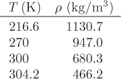
According to this table, density varies with temperature from 1130.7 kg/m3 at 216.6 K to 466.2 kg/m3 at 304.2 K. The calculated value corresponds approximately to 285 K.
Comments The calculation based on the intermolecular potential is an estimation. It does not account for the effect of temperature (assumes that the mean distance between molecules is r* regardless of temperature) and that molecules are arranged in a regular cubic lattice. Nonetheless, the final result is of the correct order of magnitude, a quite impressive result given the minimal information used in the calculation.
Ideal-Gas State
Figure 1-3 shows that at distances larger than about 10 Å the potential of carbon dioxide is fairly flat and the molecular force nearly zero. If carbon dioxide is brought to a state such that the mean distance between molecules is more than 10 Å we expect that molecules would hardly register the presence of each other and would largely move independently of each other, except for brief close encounters. This state can be reproduced experimentally by decreasing pressure (increasing volume) while keeping temperature the same. This is called the ideal-gas state. It is a state—not a gas—and is reached by any gas when pressure is reduced sufficiently. In the ideal-gas state molecules move independently of each other and without the influence of the intermolecular potential. Certain properties in this state become universal for all gases regardless of the chemical identity of their molecules. The most important example is the ideal-gas law, which describes the pressure-volume-temperature relationship of any gas at low pressures.
1.2 Statistical versus Classical Thermodynamics
Historically, a large part of thermodynamics was developed before the emergence of atomic and molecular theories of matter. This part has come to be known as classical thermodynamics and makes no reference to molecular concepts. It is based on two basic principles (“laws”) and produces a rigorous mathematical formalism that provides exact relationships between properties and forms the basis for numerical calculations. It is a credit to the ingenuity of the early developers of thermodynamics that they were capable of developing a correct theory without the benefit of molecular concepts to provide them with physical insight and guidance. The limitation is that classical thermodynamics cannot explain why a property has the value it does, nor can it provide a convincing physical explanation for the various mathematical relationships. This missing part is provided by statistical thermodynamics. The distinction between classical and statistical thermodynamics is partly artificial, partly pedagogical. Artificial, because thermodynamics makes physical sense only when we consider the molecular phenomena that produce the observed behaviors. From a pedagogical perspective, however, a proper statistical treatment requires more time to develop, which leaves less time to devote to important engineering applications. It is beyond the scope of this book to provide a bottom-up development of thermodynamics from the molecular level to the macroscopic. Instead, our goal is to develop the knowledge, skills, and confidence to perform thermodynamic calculations in chemical engineering settings. We will use molecular concepts throughout the book to shed light to new concepts but the overall development will remain under the general umbrella of classical thermodynamics. Those who wish to pursue the connection between the microscopic and the macroscopic in more detail, a subject that fascinated some of the greatest scientific minds, including Einstein, should plan to take an upper-level course in statistical mechanics from a chemical engineering, physics, or chemistry program.
The Laws of Classical Thermodynamics
Thermodynamics is built on a small number of axiomatic statements, propositions that we hold to be true on the basis of our experience with the physical world. Statistical and classical thermodynamics make use of different axiomatic statements; the axioms of statistical thermodynamics have their basis on statistical concepts; those of classical thermodynamics are based on behavior that we observe macroscopically. There are two fundamental principles in classical thermodynamics, commonly known as the first and second law.3 The first law expresses the principle that matter has the ability to store energy within. Within the context of classical thermodynamics, this is an axiomatic statement since its physical explanation is inherently molecular. The second law of thermodynamics expresses the principle that all systems, if left undisturbed, will move towards equilibrium –never away from it. This is taken as an axiomatic principle because we cannot prove it without appealing to other axiomatic statements. Nonetheless, contact with the physical world convinces us that this principle has the force a universal physical law.
3. The term law comes to us from the early days of science, a time during which scientists began to recognize mathematical order behind what had seemed up until then to be a complicated physical world that defies prediction. Many of the early scientific findings were known as “laws,” often associated with the name of the scientist who reported them, for example, Dalton’s law, Ohm’s law, Mendel’s law, etc. This practice is no longer followed. For instance, no one refers to Einstein’s famous result, E = mc2, as Einstein’s law.
Other laws of thermodynamics are often mentioned. The “zeroth” law states that, if two systems are in thermal equilibrium with a third system, they are in equilibrium with each other. The third law makes statements about the thermodynamic state at absolute zero temperature. For the purposes of our development, the first and second law are the only two principles needed in order to construct the entire mathematical theory of thermodynamics. Indeed, these are the only two equations that one must memorize in thermodynamics; all else is a matter of definitions and standard mathematical manipulations.
The “How” and the “Why” in Thermodynamics
Engineers must be skilled in the art of how to perform the required calculations, but to build confidence in the use of theoretical tools it is also important to have a sense why our methods work. The “why” in thermodynamics comes from two sources. One is physical: the molecular picture that gives meaning to “invisible” quantities such as heat, temperature, entropy, equilibrium. The other is mathematical and is expressed through exact relationships that connect the various quantities. The typical development of thermodynamics goes like this:
(a) Use physical principles to establish fundamental relationships between key properties. These relationships are obtained by applying the first and second law to the problem at hand.
(b) Use calculus to convert the fundamental relationships from step (a) into useful expressions that can be used to compute the desired quantities.
Physical intuition is needed in order to justify the fundamental relationships in step (a). Once the physical problem is converted into a mathematical one (step [b]), physical intuition is no longer needed and the gear must shift to mastering the “how.” At this point, a good handle of calculus becomes indispensable, in fact, a prerequisite for the successful completion of this material. Especially important is familiarity with functions of multiple variables, partial derivatives and path integrations.
Leave a Reply