PLOTTING THE EQUATION

Excel has very good plotting capabilities. Unfortunately, it is not possible in Excel to simply give a command such as plot(f(x)). It is necessary to produce a list or table of x and f(x) values and to graph the resulting data. This is best illustrated by an example.

Example 1.1: Plotting the Equation

A table of data and an Excel graph of the van der Waals equation for ammonia at 250°C and 10 atm are shown in Figure 1.1.

From the graph, it is easy to see that there is one real root between 0 and 5 (the other roots are complex conjugates). Remember that the van der Walls equation of state is an attempt to model the nonideality of the gas. Since the given temperature and pressure are not severe, it is expected that the calculated molar volume from the equation of state should not be greatly different from that predicted by the ideal gas law. From the ideal gas law, the molar volume is 4.29 L/gmol, which is very close to the root shown in the graph.

1.2.2 FIXED-POINT ITERATION (DIRECT SUBSTITUTION)

To apply this method, the equation must be cast into the form

x = g(x)

or, more generally,

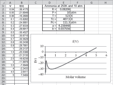
FIGURE 1.1 Roots of the van der Walls equation for ammonia at 250°C and 10 atm.

where k is an iteration counter.

Example 1.2: Direct Substitution

Note that this can always be accomplished by adding x to each side of f(x) = 0, if necessary. The van der Walls equation can be cast into the following form:

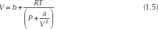
The pertinent data for ammonia are shown in Figure 1.1. If a value for V = 4 is guessed (based on the graph of Figure 1.1) and is used on the right-hand side, a new (and hopefully better) value is calculated from Equation 1.5. The iterations produce the following sequence:

4.00000 4.21854 4.22946 4.22996 4.22998.

The solution is 4.22998 L/gmol. If more significant digits are required, then more iterations can be carried out.

It should be noted that direct substitution can be a divergent process. That is, the successively calculated values actually get worse rather than closer to the correct value. Without proof, the following statements apply:

Let g΄ be the first derivative of the function g in Equation 1.4. Then,

• If |g΄| < 1, the error will decrease with each iteration.

• If |g΄| > 1, the error grows at each iteration.

• If g΄ > 0, the error will have the same sign at each iteration.

• If g΄ < 0, the error will alternate signs at each iteration.

Clearly, the equation should be arranged so that the magnitude of g΄ is less than 1. This might take some experimentation. Often, a form of g is tried, and if the process does not converge, then other forms are attempted.