Many engineering problems require the solution of a single nonlinear equation. Such an equation can always be cast into the form

The objective of this chapter is to study methods and learn of Excel^® tools for finding the root(s) of a nonlinear equation, that is, for finding x such that f(x) = 0.

Simple algebra provides the root for a linear equation. However, for more complex (nonlinear or transcendental) equations, it is often the case that no analytical solution is available, or is difficult to obtain, so that numerical methods must be used.

An example of a nonlinear equation is the van der Waals equation of state, which is given by

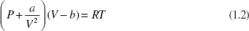
where

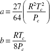
with subscript c referring to the “critical” values of temperature and pressure for the gas. Note that, if a and b are zero, this reduces to the ideal gas equation of state.

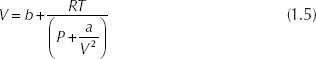
A typical problem is to find the molar volume, V, given the temperature and pressure (and the type of gas). While it is possible to find analytic solutions to the van der Waals equation of state for V (this is simply a cubic equation), a numerical solution is often preferred. The equation of state in the form f(x) = 0 is obtained by simple rearrangement:

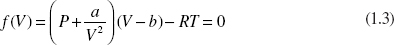
Note that this particular form f(x) = 0 is not unique, and other algebraic rearrangements are possible.

1.2 ALGORITHMS FOR SOLVING f(x) = 0

Clearly there is a need to find good methods for determining roots. Four such methods are now presented (though many more have been developed): fixed-point iteration (direct substitution), bisection, Newton’s method, and the secant method. These methods are iterative. That is, given a guess of a root, or the interval in which a root lies, the algorithm refines that guess repeatedly, obtaining (hopefully) better and better guesses, until a value “close enough” to the true root is found. Also, graphing the equation can add insight into the roots of interest and can provide good initial estimates of the roots for the iterative algorithms. It is recommended to always prepare a graph of the function to give insight into possible solutions.

1.2.1 PLOTTING THE EQUATION

Excel has very good plotting capabilities. Unfortunately, it is not possible in Excel to simply give a command such as plot(f(x)). It is necessary to produce a list or table of x and f(x) values and to graph the resulting data. This is best illustrated by an example.

Example 1.1: Plotting the Equation

A table of data and an Excel graph of the van der Waals equation for ammonia at 250°C and 10 atm are shown in Figure 1.1.

From the graph, it is easy to see that there is one real root between 0 and 5 (the other roots are complex conjugates). Remember that the van der Walls equation of state is an attempt to model the nonideality of the gas. Since the given temperature and pressure are not severe, it is expected that the calculated molar volume from the equation of state should not be greatly different from that predicted by the ideal gas law. From the ideal gas law, the molar volume is 4.29 L/gmol, which is very close to the root shown in the graph.

1.2.2 FIXED-POINT ITERATION (DIRECT SUBSTITUTION)

To apply this method, the equation must be cast into the form

x = g(x)

or, more generally,

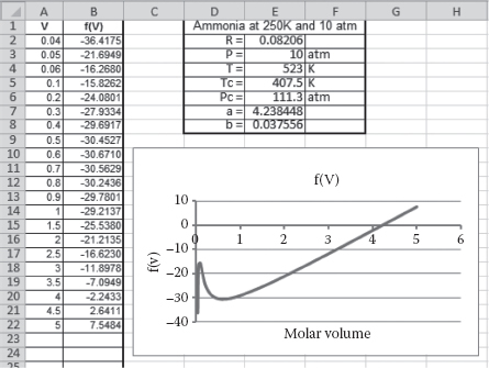
FIGURE 1.1 Roots of the van der Walls equation for ammonia at 250°C and 10 atm.

where k is an iteration counter.

Example 1.2: Direct Substitution

Note that this can always be accomplished by adding x to each side of f(x) = 0, if necessary. The van der Walls equation can be cast into the following form:

The pertinent data for ammonia are shown in Figure 1.1. If a value for V = 4 is guessed (based on the graph of Figure 1.1) and is used on the right-hand side, a new (and hopefully better) value is calculated from Equation 1.5. The iterations produce the following sequence:

4.00000 4.21854 4.22946 4.22996 4.22998.

The solution is 4.22998 L/gmol. If more significant digits are required, then more iterations can be carried out.

It should be noted that direct substitution can be a divergent process. That is, the successively calculated values actually get worse rather than closer to the correct value. Without proof, the following statements apply:

Let g΄ be the first derivative of the function g in Equation 1.4. Then,

• If |g΄| < 1, the error will decrease with each iteration.

• If |g΄| > 1, the error grows at each iteration.

• If g΄ > 0, the error will have the same sign at each iteration.

• If g΄ < 0, the error will alternate signs at each iteration.

Clearly, the equation should be arranged so that the magnitude of g΄ is less than 1. This might take some experimentation. Often, a form of g is tried, and if the process does not converge, then other forms are attempted.

1.2.3 BISECTION

If it is (somehow) known that a root lies in the interval [a, b], then by simply halving the interval in which the root lies, the interval can be reduced to an acceptable level. This idea is at the heart of the bisection method as shown in Figure 1.2.

The restriction is that f(a) and f(b) must have opposite signs—one of them must be positive, the other negative (it does not matter which). Then, because f is assumed to be continuous, it must be a zero somewhere in [a, b]. Let c be the midpoint of [a, b]. Either c is the root, or the root lies in [a, c] or in [a, b]. If f(c) is close enough to zero (see below regarding tolerance), then the root has been found. Otherwise, one pair of [f(a),f(c)]or [f(c),f(b)] has opposite signs. Keep the half-interval with opposite signs and discard the other. Repeat the process until either (1) f, evaluated at the midpoint of the interval, is sufficiently small or (2) the interval has been shrunk to a suitably small value.

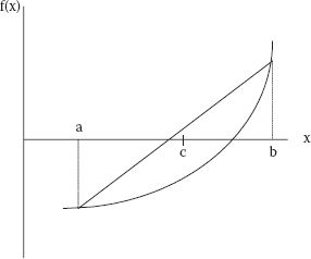
FIGURE 1.2 Bisection: c = (a + b)/2.

The term “sufficiently small” is usually tested using a “tolerance,” which represents a number small enough to be considered zero based on the application. This can be stated more formally as follows:

If |f(x)|<tolerance then (x) is sufficiently small.

Example 1.3: Bisection Applied to the van der Waals EOS

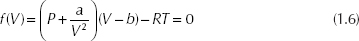
Recall the van der Waals EOS in the form

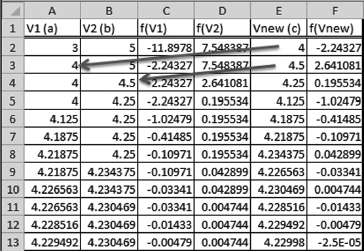
The table below shows the progression of applying the bisection method. It uses the Excel IF function to choose whether f(a) or f(b) is replaced by f(c) (and correspondingly whether a or b is to be replaced by c). The syntax for the IF function is as follows (see the explanation of the Excel spreadsheet below for a full explanation of how the IF function is used):

IF(test, True Value, False Value)

In this example (again for ammonia at 10 atm and 250°C), the function in the cell below the label V1 (corresponding to the point a in the nomenclature of the figure) is = IF(F2<0, E2, A2), where cell F3 holds f(Vnew) [corresponding to f(c)], E2 contains Vnew (corresponding to c), and A2 holds V1. So, if f(Vnew) is negative (test is TRUE), V1 (corresponding to a) gets the Vnew value; otherwise, it retains the old V1. Likewise, the formula in the cell below the V2 label is = IF(F2<0,B2,E2), which replaces V2 (corresponding to b) with the value Vnew if the test (F2 < 0) is FALSE. After the first row of formulas has been entered, these cells are copied down to repeat the iterations. Iterations should be repeated until f(Vnew) is sufficiently small (in absolute value). The initial guesses for V are 3 and 5, respectively, which give opposite signs for the function.

Did You Know?: That there are two ways to copy cell contents down. One way is to select the cells to be copied and then grab the small box in the lower right corner of the selection. Pulling down will copy the cells. The second method is to select the cells to be copied and while holding down the mouse button pull down as far as desired and finally hitting CTRL/d (hold down the CTRL key and hit the d key).

1.2.4 NEWTON’S METHOD

The next algorithm to be considered is the Newton’s method for finding roots. Newton’s method does not always converge. But, when it does converge, it usually does so very rapidly (at least once it is “close enough” to the root). Newton’s method also has the advantage of not requiring a bracketing interval with positive and negative values. So Newton’s method allows the solution of equations such as

whereas bisection does not. This parabola just touches the zero axis and has no negative values.

The basic idea of the Newton algorithm is this: given an initial guess, call it x¹ to a root of f(x) = 0, a refined guess, x², is computed based on the x-intercept of the line tangent to f(x) at x¹. That is, consider the equation of the line tangent to f(x) at x¹ (this is just the Taylor series expansion of the function ignoring all but linear terms):

This is the point-slope equation of a line, where x¹ is the base point and f΄(x¹) is the slope [derivative of f(x) evaluated at x¹]. Solving Equation 1.8 for x at which f(x) = 0 gives

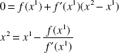
or more generally,

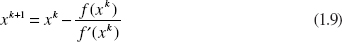
The value of x^k+1 is the new guess at the root. The process is repeated, computing successively x², x³, x⁴,… until an x^K is found at which

where tol is a prescribed tolerance.

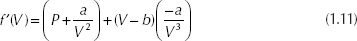
Example 1.4: Newton’s Method Applied to the van der Waals Equation

Newton’s method is now applied for ammonia at 10 atm and 250°C with an initial guess for V = 1 L/gmol. To begin using Newton’s method, the derivative of Equation 1.2 is required and is as follows:

Here is an Excel spreadsheet that solves this problem:

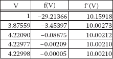
The root is found in about 3 iterations. Note the rapid rate of convergence.

An examination of Equation 1.9 for the new iterate x^k reveals a potential for failure of Newton’s method, namely,

This may lead to a wildly divergent iterative process. There are other possible reasons why this method might not converge. In general, Newton’s method is prone to failure, but when it does work, it converges rapidly. Good initial guesses are the key to success.