Category: Matlab

  • Data Output

    Data export (or output) in MATLAB means to write into files. MATLAB allows you to use your data in another application that reads ASCII files. For this, MATLAB provides several data export options.

    You can create the following type of files −

    • Rectangular, delimited ASCII data file from an array.
    • Diary (or log) file of keystrokes and the resulting text output.
    • Specialized ASCII file using low-level functions such as fprintf.
    • MEX-file to access your C/C++ or Fortran routine that writes to a particular text file format.

    Apart from this, you can also export data to spreadsheets.

    There are two ways to export a numeric array as a delimited ASCII data file −

    • Using the save function and specifying the -ascii qualifier
    • Using the dlmwrite function

    Syntax for using the save function is −

    save my_data.out num_array -ascii
    

    where, my_data.out is the delimited ASCII data file created, num_array is a numeric array and −ascii is the specifier.

    Syntax for using the dlmwrite function is −

    dlmwrite('my_data.out', num_array, 'dlm_char')
    

    where, my_data.out is the delimited ASCII data file created, num_array is a numeric array and dlm_char is the delimiter character.

    Example

    The following example demonstrates the concept. Create a script file and type the following code −

    num_array = [ 1 2 3 4 ; 4 5 6 7; 7 8 9 0];
    save array_data1.out num_array -ascii;
    type array_data1.out
    dlmwrite('array_data2.out', num_array, ' ');
    type array_data2.out

    When you run the file, it displays the following result −

       1.0000000e+00   2.0000000e+00   3.0000000e+00   4.0000000e+00
       4.0000000e+00   5.0000000e+00   6.0000000e+00   7.0000000e+00
       7.0000000e+00   8.0000000e+00   9.0000000e+00   0.0000000e+00
    
    1 2 3 4
    4 5 6 7
    7 8 9 0
    

    Please note that the save -ascii command and the dlmwrite function does not work with cell arrays as input. To create a delimited ASCII file from the contents of a cell array, you can

    • Either, convert the cell array to a matrix using the cell2mat function
    • Or export the cell array using low-level file I/O functions.

    If you use the save function to write a character array to an ASCII file, it writes the ASCII equivalent of the characters to the file.

    For example, let us write the word ‘hello’ to a file −

    h = 'hello';
    save textdata.out h -ascii
    type textdata.out

    MATLAB executes the above statements and displays the following result. which is the characters of the string ‘hello’ in 8-digit ASCII format.

    1.0400000e+02   1.0100000e+02   1.0800000e+02   1.0800000e+02   1.1100000e+02
    

    Writing to Diary Files

    Diary files are activity logs of your MATLAB session. The diary function creates an exact copy of your session in a disk file, excluding graphics.

    To turn on the diary function, type −

    diary

    Optionally, you can give the name of the log file, say −

    diary logdata.out
    

    To turn off the diary function −

    diary off
    

    You can open the diary file in a text editor.

    Exporting Data to Text Data Files with Low-Level I/O

    So far, we have exported numeric arrays. However, you may need to create other text files, including combinations of numeric and character data, nonrectangular output files, or files with non-ASCII encoding schemes. For these purposes, MATLAB provides the low-level fprintf function.

    As in low-level I/O file activities, before exporting, you need to open or create a file with the fopen function and get the file identifier. By default, fopen opens a file for read-only access. You should specify the permission to write or append, such as ‘w’ or ‘a’.

    After processing the file, you need to close it with fclose(fid) function.

    The following example demonstrates the concept −

    Example

    Create a script file and type the following code in it −

    % create a matrix y, with two rows
    x = 0:10:100;
    y = [x; log(x)];
     
    % open a file for writing
    fid = fopen('logtable.txt', 'w');
     
    % Table Header
    fprintf(fid, 'Log     Function\n\n');
     
    % print values in column order
    % two values appear on each row of the file
    fprintf(fid, '%f    %f\n', y);
    fclose(fid);
    
    % display the file created
    type logtable.txt

    When you run the file, it displays the following result −

    Log         Function
    
    0.000000    -Inf
    10.000000    2.302585
    20.000000    2.995732
    30.000000    3.401197
    40.000000    3.688879
    50.000000    3.912023
    60.000000    4.094345
    70.000000    4.248495
    80.000000    4.382027
    90.000000    4.499810
    100.000000    4.605170
    
  • Data Import

    Importing data in MATLAB means loading data from an external file. The importdata function allows loading various data files of different formats. It has the following five forms −

    Sr.No.Function & Description
    1A = importdata(filename)Loads data into array A from the file denoted by filename.
    2A = importdata(‘-pastespecial’)Loads data from the system clipboard rather than from a file.
    3A = importdata(___, delimiterIn)Interprets delimiterIn as the column separator in ASCII file, filename, or the clipboard data. You can use delimiterIn with any of the input arguments in the above syntaxes.
    4A = importdata(___, delimiterIn, headerlinesIn)Loads data from ASCII file, filename, or the clipboard, reading numeric data starting from line headerlinesIn+1.
    5[A, delimiterOut, headerlinesOut] = importdata(___)Returns the detected delimiter character for the input ASCII file in delimiterOut and the detected number of header lines in headerlinesOut, using any of the input arguments in the previous syntaxes.

    By default, Octave does not have support for importdata() function, so you will have to search and install this package to make following examples work with your Octave installation.

    Example 1

    Let us load and display an image file. Create a script file and type the following code in it −

    filename = 'smile.jpg';
    A = importdata(filename);
    image(A);

    When you run the file, MATLAB displays the image file. However, you must store it in the current directory.

    Importing Imange Files

    Example 2

    In this example, we import a text file and specify Delimiter and Column Header. Let us create a space-delimited ASCII file with column headers, named weeklydata.txt.

    Our text file weeklydata.txt looks like this −

    SunDay  MonDay  TuesDay  WednesDay  ThursDay  FriDay  SaturDay
    95.01   76.21   61.54    40.57       55.79    70.28   81.53
    73.11   45.65   79.19    93.55       75.29    69.87   74.68
    60.68   41.85   92.18    91.69       81.32    90.38   74.51
    48.60   82.14   73.82    41.03       0.99     67.22   93.18
    89.13   44.47   57.63    89.36       13.89    19.88   46.60
    

    Create a script file and type the following code in it −

    filename = 'weeklydata.txt';
    delimiterIn = ' ';
    headerlinesIn = 1;
    A = importdata(filename,delimiterIn,headerlinesIn);
    
    % View data
    for k = [1:7]
       disp(A.colheaders{1, k})
       disp(A.data(:, k))
       disp(' ')
    end

    When you run the file, it displays the following result −

    SunDay
       95.0100
       73.1100
       60.6800
       48.6000
       89.1300
     
    MonDay
       76.2100
       45.6500
       41.8500
       82.1400
       44.4700
     
    TuesDay
       61.5400
       79.1900
       92.1800
       73.8200
       57.6300
    
    WednesDay
       40.5700
       93.5500
       91.6900
       41.0300
       89.3600
     
    ThursDay
       55.7900
       75.2900
       81.3200
       0.9900
       13.8900
     
    FriDay
       70.2800
       69.8700
       90.3800
       67.2200
       19.8800
    
    SaturDay
       81.5300
       74.6800
       74.5100
       93.1800
       46.6000
    

    Example 3

    In this example, let us import data from clipboard.

    Copy the following lines to the clipboard −

    Mathematics is simple

    Create a script file and type the following code −

    A = importdata('-pastespecial')
    

    When you run the file, it displays the following result −

    A = 
       'Mathematics is simple'
    

    Low-Level File I/O

    The importdata function is a high-level function. The low-level file I/O functions in MATLAB allow the most control over reading or writing data to a file. However, these functions need more detailed information about your file to work efficiently.

    MATLAB provides the following functions for read and write operations at the byte or character level −

    FunctionDescription
    fcloseClose one or all open files
    feofTest for end-of-file
    ferrorInformation about file I/O errors
    fgetlRead line from file, removing newline characters
    fgetsRead line from file, keeping newline characters
    fopenOpen file, or obtain information about open files
    fprintfWrite data to text file
    freadRead data from binary file
    frewindMove file position indicator to beginning of open file
    fscanfRead data from text file
    fseekMove to specified position in file
    ftellPosition in open file
    fwriteWrite data to binary file

    Import Text Data Files with Low-Level I/O

    MATLAB provides the following functions for low-level import of text data files −

    • The fscanf function reads formatted data in a text or ASCII file.
    • The fgetl and fgets functions read one line of a file at a time, where a newline character separates each line.
    • The fread function reads a stream of data at the byte or bit level.

    Example

    We have a text data file ‘myfile.txt’ saved in our working directory. The file stores rainfall data for three months; June, July and August for the year 2012.

    The data in myfile.txt contains repeated sets of time, month and rainfall measurements at five places. The header data stores the number of months M; so we have M sets of measurements.

    The file looks like this −

    Rainfall Data
    Months: June, July, August
     
    M = 3
    12:00:00
    June-2012
    17.21  28.52  39.78  16.55 23.67
    19.15  0.35   17.57  NaN   12.01
    17.92  28.49  17.40  17.06 11.09
    9.59   9.33   NaN    0.31  0.23 
    10.46  13.17  NaN    14.89 19.33
    20.97  19.50  17.65  14.45 14.00
    18.23  10.34  17.95  16.46 19.34
    09:10:02
    July-2012
    12.76  16.94  14.38  11.86 16.89
    20.46  23.17  NaN    24.89 19.33
    30.97  49.50  47.65  24.45 34.00
    18.23  30.34  27.95  16.46 19.34
    30.46  33.17  NaN    34.89  29.33
    30.97  49.50  47.65  24.45 34.00
    28.67  30.34  27.95  36.46 29.34
    15:03:40
    August-2012
    17.09  16.55  19.59  17.25 19.22
    17.54  11.45  13.48  22.55 24.01
    NaN    21.19  25.85  25.05 27.21
    26.79  24.98  12.23  16.99 18.67
    17.54  11.45  13.48  22.55 24.01
    NaN    21.19  25.85  25.05 27.21
    26.79  24.98  12.23  16.99 18.67
    

    We will import data from this file and display this data. Take the following steps −

    • Open the file with fopen function and get the file identifier.
    • Describe the data in the file with format specifiers, such as ‘%s‘ for a string, ‘%d‘ for an integer, or ‘%f‘ for a floating-point number.
    • To skip literal characters in the file, include them in the format description. To skip a data field, use an asterisk (‘*’) in the specifier.For example, to read the headers and return the single value for M, we write −M = fscanf(fid, ‘%*s %*s\n%*s %*s %*s %*s\nM=%d\n\n’, 1);
    • By default, fscanf reads data according to our format description until it does not find any match for the data, or it reaches the end of the file. Here we will use for loop for reading 3 sets of data and each time, it will read 7 rows and 5 columns.
    • We will create a structure named mydata in the workspace to store data read from the file. This structure has three fields – timemonth, and raindata array.

    Create a script file and type the following code in it −

    filename = '/data/myfile.txt';
    rows = 7;
    cols = 5;
     
    % open the file
    fid = fopen(filename);
     
    % read the file headers, find M (number of months)
    M = fscanf(fid, '%*s %*s\n%*s %*s %*s %*s\nM=%d\n\n', 1);
     
    % read each set of measurements
    for n = 1:M
       mydata(n).time = fscanf(fid, '%s', 1);
       mydata(n).month = fscanf(fid, '%s', 1);
     
       % fscanf fills the array in column order,
       % so transpose the results
       mydata(n).raindata  = ...
    
      fscanf(fid, '%f', [rows, cols]);
    end for n = 1:M disp(mydata(n).time), disp(mydata(n).month) disp(mydata(n).raindata) end % close the file fclose(fid);

    When you run the file, it displays the following result −

    12:00:00
    June-2012
       17.2100   17.5700   11.0900   13.1700   14.4500
       28.5200       NaN    9.5900       NaN   14.0000
       39.7800   12.0100    9.3300   14.8900   18.2300
       16.5500   17.9200       NaN   19.3300   10.3400
       23.6700   28.4900    0.3100   20.9700   17.9500
       19.1500   17.4000    0.2300   19.5000   16.4600
       0.3500   17.0600   10.4600   17.6500   19.3400
    
    09:10:02
    July-2012
       12.7600       NaN   34.0000   33.1700   24.4500
       16.9400   24.8900   18.2300       NaN   34.0000
       14.3800   19.3300   30.3400   34.8900   28.6700
       11.8600   30.9700   27.9500   29.3300   30.3400
       16.8900   49.5000   16.4600   30.9700   27.9500
       20.4600   47.6500   19.3400   49.5000   36.4600
       23.1700   24.4500   30.4600   47.6500   29.3400
    
    15:03:40
    August-2012
       17.0900   13.4800   27.2100   11.4500   25.0500
       16.5500   22.5500   26.7900   13.4800   27.2100
       19.5900   24.0100   24.9800   22.5500   26.7900
       17.2500       NaN   12.2300   24.0100   24.9800
       19.2200   21.1900   16.9900       NaN   12.2300
       17.5400   25.8500   18.6700   21.1900   16.9900
       11.4500   25.0500   17.5400   25.8500   18.6700
    
  • Functions

    A function is a group of statements that together perform a task. In MATLAB, functions are defined in separate files. The name of the file and of the function should be the same.

    Functions operate on variables within their own workspace, which is also called the local workspace, separate from the workspace you access at the MATLAB command prompt which is called the base workspace.

    Functions can accept more than one input arguments and may return more than one output arguments.

    Syntax of a function statement is −

    function [out1,out2, ..., outN] = myfun(in1,in2,in3, ..., inN)
    

    Example

    The following function named mymax should be written in a file named mymax.m. It takes five numbers as argument and returns the maximum of the numbers.

    Create a function file, named mymax.m and type the following code in it −

    function max = mymax(n1, n2, n3, n4, n5)
    
    %This function calculates the maximum of the
    % five numbers given as input
    max =  n1;
    if(n2 > max)
       max = n2;
    end
    if(n3 > max)
       max = n3;
    end
    if(n4 > max)
       max = n4;
    end
    if(n5 > max)
       max = n5;
    end

    The first line of a function starts with the keyword function. It gives the name of the function and order of arguments. In our example, the mymax function has five input arguments and one output argument.

    The comment lines that come right after the function statement provide the help text. These lines are printed when you type −

    help mymax
    

    MATLAB will execute the above statement and return the following result −

    This function calculates the maximum of the
       five numbers given as input
    

    You can call the function as −

    mymax(34, 78, 89, 23, 11)
    

    MATLAB will execute the above statement and return the following result −

    ans = 89
    

    Anonymous Functions

    An anonymous function is like an inline function in traditional programming languages, defined within a single MATLAB statement. It consists of a single MATLAB expression and any number of input and output arguments.

    You can define an anonymous function right at the MATLAB command line or within a function or script.

    This way you can create simple functions without having to create a file for them.

    The syntax for creating an anonymous function from an expression is

    f = @(arglist)expression
    

    Example

    In this example, we will write an anonymous function named power, which will take two numbers as input and return first number raised to the power of the second number.

    Create a script file and type the following code in it −

    power = @(x, n) x.^n;
    result1 = power(7, 3)
    result2 = power(49, 0.5)
    result3 = power(10, -10)
    result4 = power (4.5, 1.5)

    When you run the file, it displays −

    result1 =  343
    result2 =  7
    result3 =  1.0000e-10
    result4 =  9.5459
    

    Primary and Sub-Functions

    Any function other than an anonymous function must be defined within a file. Each function file contains a required primary function that appears first and any number of optional sub-functions that comes after the primary function and used by it.

    Primary functions can be called from outside of the file that defines them, either from command line or from other functions, but sub-functions cannot be called from command line or other functions, outside the function file.

    Sub-functions are visible only to the primary function and other sub-functions within the function file that defines them.

    Example

    Let us write a function named quadratic that would calculate the roots of a quadratic equation. The function would take three inputs, the quadratic co-efficient, the linear co-efficient and the constant term. It would return the roots.

    The function file quadratic.m will contain the primary function quadratic and the sub-function disc, which calculates the discriminant.

    Create a function file quadratic.m and type the following code in it −

    function [x1,x2] = quadratic(a,b,c)
    
    %this function returns the roots of 
    % a quadratic equation.
    % It takes 3 input arguments
    % which are the co-efficients of x2, x and the 
    %constant term
    % It returns the roots
    d = disc(a,b,c); 
    x1 = (-b + d) / (2*a);
    x2 = (-b - d) / (2*a);
    end   % end of quadratic
    
    function dis = disc(a,b,c) 
    %function calculates the discriminant
    dis = sqrt(b^2 - 4*a*c);
    end   % end of sub-function

    You can call the above function from command prompt as −

    quadratic(2,4,-4)

    MATLAB will execute the above statement and return the following result −

    ans = 0.7321
    

    Nested Functions

    You can define functions within the body of another function. These are called nested functions. A nested function contains any or all of the components of any other function.

    Nested functions are defined within the scope of another function and they share access to the containing function’s workspace.

    A nested function follows the following syntax −

    function x = A(p1, p2)
    ...
    B(p2)
       function y = B(p3)
       ...
       end
    ...
    end
    

    Example

    Let us rewrite the function quadratic, from previous example, however, this time the disc function will be a nested function.

    Create a function file quadratic2.m and type the following code in it −

    function [x1,x2] = quadratic2(a,b,c)
    function disc  % nested function
    d = sqrt(b^2 - 4*a*c);
    end   % end of function disc
    
    disc;
    x1 = (-b + d) / (2*a);
    x2 = (-b - d) / (2*a);
    end   % end of function quadratic2

    You can call the above function from command prompt as −

    quadratic2(2,4,-4)

    MATLAB will execute the above statement and return the following result −

    ans =  0.73205
    

    Private Functions

    A private function is a primary function that is visible only to a limited group of other functions. If you do not want to expose the implementation of a function(s), you can create them as private functions.

    Private functions reside in subfolders with the special name private.

    They are visible only to functions in the parent folder.

    Example

    Let us rewrite the quadratic function. This time, however, the disc function calculating the discriminant, will be a private function.

    Create a subfolder named private in working directory. Store the following function file disc.m in it −

    function dis = disc(a,b,c) 
    %function calculates the discriminant
    dis = sqrt(b^2 - 4*a*c);
    end      % end of sub-function

    Create a function quadratic3.m in your working directory and type the following code in it −

    function [x1,x2] = quadratic3(a,b,c)
    
    %this function returns the roots of 
    % a quadratic equation.
    % It takes 3 input arguments
    % which are the co-efficient of x2, x and the 
    %constant term
    % It returns the roots
    d = disc(a,b,c); 
    
    x1 = (-b + d) / (2*a);
    x2 = (-b - d) / (2*a);
    end      % end of quadratic3

    You can call the above function from command prompt as −

    quadratic3(2,4,-4)

    MATLAB will execute the above statement and return the following result −

    ans =  0.73205
    

    Global Variables

    Global variables can be shared by more than one function. For this, you need to declare the variable as global in all the functions.

    If you want to access that variable from the base workspace, then declare the variable at the command line.

    The global declaration must occur before the variable is actually used in a function. It is a good practice to use capital letters for the names of global variables to distinguish them from other variables.

    Example

    Let us create a function file named average.m and type the following code in it −

    function avg = average(nums)
    global TOTAL
    avg = sum(nums)/TOTAL;
    end

    Create a script file and type the following code in it −

    global TOTAL;
    TOTAL = 10;
    n = [34, 45, 25, 45, 33, 19, 40, 34, 38, 42];
    av = average(n)

    When you run the file, it will display the following result −

    av =  35.500
    
  • Strings

    Creating a character string is quite simple in MATLAB. In fact, we have used it many times. For example, you type the following in the command prompt −

    my_string = 'Tutorials Point'

    MATLAB will execute the above statement and return the following result −

    my_string = Tutorials Point
    

    MATLAB considers all variables as arrays, and strings are considered as character arrays. Let us use the whos command to check the variable created above −

    whos

    MATLAB will execute the above statement and return the following result −

    Name           Size            Bytes  Class    Attributes
    my_string      1x16               32  char
    

    Interestingly, you can use numeric conversion functions like uint8 or uint16 to convert the characters in the string to their numeric codes. The char function converts the integer vector back to characters −

    Example

    Create a script file and type the following code into it −

    my_string = 'Tutorial''s Point';
    str_ascii = uint8(my_string)        % 8-bit ascii values
    str_back_to_char= char(str_ascii)  
    str_16bit = uint16(my_string)       % 16-bit ascii values
    str_back_to_char = char(str_16bit)  

    When you run the file, it displays the following result −

    str_ascii =
    
       84  117  116  111  114  105   97  108   39  115   32   80  111  105  110  116
    
    str_back_to_char = Tutorial's Point
    str_16bit =
    
       84  117  116  111  114  105   97  108   39  115   32   80  111  105  110  116
    
    str_back_to_char = Tutorial's Point
    

    Rectangular Character Array

    The strings we have discussed so far are one-dimensional character arrays; however, we need to store more than that. We need to store more dimensional textual data in our program. This is achieved by creating rectangular character arrays.

    Simplest way of creating a rectangular character array is by concatenating two or more one-dimensional character arrays, either vertically or horizontally as required.

    You can combine strings vertically in either of the following ways −

    • Using the MATLAB concatenation operator [] and separating each row with a semicolon (;). Please note that in this method each row must contain the same number of characters. For strings with different lengths, you should pad with space characters as needed.
    • Using the char function. If the strings are of different lengths, char pads the shorter strings with trailing blanks so that each row has the same number of characters.

    Example

    Create a script file and type the following code into it −

    doc_profile = ['Zara Ali                             '; ...
    
               'Sr. Surgeon                          '; ...
               'R N Tagore Cardiology Research Center']
    doc_profile = char('Zara Ali', 'Sr. Surgeon', ...
                  'RN Tagore Cardiology Research Center')</code></pre>

    When you run the file, it displays the following result −

    doc_profile =
    Zara Ali                             
    Sr. Surgeon                          
    R N Tagore Cardiology Research Center
    doc_profile =
    Zara Ali                            
    Sr. Surgeon                         
    RN Tagore Cardiology Research Center
    

    You can combine strings horizontally in either of the following ways −

    • Using the MATLAB concatenation operator, [] and separating the input strings with a comma or a space. This method preserves any trailing spaces in the input arrays.
    • Using the string concatenation function, strcat. This method removes trailing spaces in the inputs.

    Example

    Create a script file and type the following code into it −

    name =     'Zara Ali                             ';
    position = 'Sr. Surgeon                          '; 
    worksAt =  'R N Tagore Cardiology Research Center';
    profile = [name ', ' position ', ' worksAt]
    profile = strcat(name, ', ', position, ', ', worksAt)

    When you run the file, it displays the following result −

    profile = Zara Ali      , Sr. Surgeon      , R N Tagore Cardiology Research Center
    profile = Zara Ali,Sr. Surgeon,R N Tagore Cardiology Research Center
    

    Combining Strings into a Cell Array

    From our previous discussion, it is clear that combining strings with different lengths could be a pain as all strings in the array has to be of the same length. We have used blank spaces at the end of strings to equalize their length.

    However, a more efficient way to combine the strings is to convert the resulting array into a cell array.

    MATLAB cell array can hold different sizes and types of data in an array. Cell arrays provide a more flexible way to store strings of varying length.

    The cellstr function converts a character array into a cell array of strings.

    Example

    Create a script file and type the following code into it −

    name =     'Zara Ali                             ';
    position = 'Sr. Surgeon                          '; 
    worksAt =  'R N Tagore Cardiology Research Center';
    profile = char(name, position, worksAt);
    profile = cellstr(profile);
    disp(profile)

    When you run the file, it displays the following result −

    {                                                                               
       [1,1] = Zara Ali                                                              
       [2,1] = Sr. Surgeon                                                           
       [3,1] = R N Tagore Cardiology Research Center                                 
    }   
    

    String Functions in MATLAB

    MATLAB provides numerous string functions creating, combining, parsing, comparing and manipulating strings.

    Following table provides brief description of the string functions in MATLAB −

    FunctionPurpose
    Functions for storing text in character arrays, combine character arrays, etc.
    blanksCreate string of blank characters
    cellstrCreate cell array of strings from character array
    charConvert to character array (string)
    iscellstrDetermine whether input is cell array of strings
    ischarDetermine whether item is character array
    sprintfFormat data into string
    strcatConcatenate strings horizontally
    strjoinJoin strings in cell array into single string
    Functions for identifying parts of strings, find and replace substrings
    ischarDetermine whether item is character array
    isletterArray elements that are alphabetic letters
    isspaceArray elements that are space characters
    isstrpropDetermine whether string is of specified category
    sscanfRead formatted data from string
    strfindFind one string within another
    strrepFind and replace substring
    strsplitSplit string at specified delimiter
    strtokSelected parts of string
    validatestringCheck validity of text string
    symvarDetermine symbolic variables in expression
    regexpMatch regular expression (case sensitive)
    regexpiMatch regular expression (case insensitive)
    regexprepReplace string using regular expression
    regexptranslateTranslate string into regular expression
    Functions for string comparison
    strcmpCompare strings (case sensitive)
    strcmpiCompare strings (case insensitive)
    strncmpCompare first n characters of strings (case sensitive)
    strncmpiCompare first n characters of strings (case insensitive)
    Functions for changing string to upper- or lowercase, creating or removing white space
    deblankStrip trailing blanks from end of string
    strtrimRemove leading and trailing white space from string
    lowerConvert string to lowercase
    upperConvert string to uppercase
    strjustJustify character array

    Examples

    The following examples illustrate some of the above-mentioned string functions −

    Formatting Strings

    Create a script file and type the following code into it −

    A = pi*1000*ones(1,5);
    sprintf(' %f \n %.2f \n %+.2f \n %12.2f \n %012.2f \n', A)

    When you run the file, it displays the following result −

    ans =  3141.592654 
       3141.59 
       +3141.59 
    
      3141.59 
    000003141.59

    Joining Strings

    Create a script file and type the following code into it −

    %cell array of strings
    str_array = {'red','blue','green', 'yellow', 'orange'};
    
    % Join strings in cell array into single string
    str1 = strjoin(str_array, "-")
    str2 = strjoin(str_array, ",")

    When you run the file, it displays the following result −

    str1 = red-blue-green-yellow-orange
    str2 = red,blue,green,yellow,orange
    

    Finding and Replacing Strings

    Create a script file and type the following code into it −

    students = {'Zara Ali', 'Neha Bhatnagar', ...
    
            'Monica Malik', 'Madhu Gautam', ...
            'Madhu Sharma', 'Bhawna Sharma',...
            'Nuha Ali', 'Reva Dutta', ...
            'Sunaina Ali', 'Sofia Kabir'};
    % The strrep function searches and replaces sub-string. new_student = strrep(students(8), 'Reva', 'Poulomi') % Display first names first_names = strtok(students)

    When you run the file, it displays the following result −

    new_student = 
    {
       [1,1] = Poulomi Dutta
    }
    first_names = 
    {
       [1,1] = Zara
       [1,2] = Neha
       [1,3] = Monica
       [1,4] = Madhu
       [1,5] = Madhu
       [1,6] = Bhawna
       [1,7] = Nuha
       [1,8] = Reva
       [1,9] = Sunaina
       [1,10] = Sofia
    }
    

    Comparing Strings

    Create a script file and type the following code into it −

    str1 = 'This is test'
    str2 = 'This is text'
    if (strcmp(str1, str2))
       sprintf('%s and %s are equal', str1, str2)
    else
       sprintf('%s and %s are not equal', str1, str2)
    end

    When you run the file, it displays the following result −

    str1 = This is test
    str2 = This is text
    ans = This is test and This is text are not equal
    
  • Numbers

    MATLAB supports various numeric classes that include signed and unsigned integers and single-precision and double-precision floating-point numbers. By default, MATLAB stores all numeric values as double-precision floating point numbers.

    You can choose to store any number or array of numbers as integers or as single-precision numbers.

    All numeric types support basic array operations and mathematical operations.

    Conversion to Various Numeric Data Types

    MATLAB provides the following functions to convert to various numeric data types −

    FunctionPurpose
    doubleConverts to double precision number
    singleConverts to single precision number
    int8Converts to 8-bit signed integer
    int16Converts to 16-bit signed integer
    int32Converts to 32-bit signed integer
    int64Converts to 64-bit signed integer
    uint8Converts to 8-bit unsigned integer
    uint16Converts to 16-bit unsigned integer
    uint32Converts to 32-bit unsigned integer
    uint64Converts to 64-bit unsigned integer

    Example

    Create a script file and type the following code −

    x = single([5.32 3.47 6.28]) .* 7.5
    x = double([5.32 3.47 6.28]) .* 7.5
    x = int8([5.32 3.47 6.28]) .* 7.5
    x = int16([5.32 3.47 6.28]) .* 7.5
    x = int32([5.32 3.47 6.28]) .* 7.5
    x = int64([5.32 3.47 6.28]) .* 7.5

    When you run the file, it shows the following result −

    x =
    
       39.900   26.025   47.100
    
    x =
    
       39.900   26.025   47.100
    
    x =
    
       38  23  45
    
    x =
    
       38  23  45
    
    x =
    
       38  23  45
    
    x =
    
       38  23  45
    

    Example

    Let us extend the previous example a little more. Create a script file and type the following code −

    x = int32([5.32 3.47 6.28]) .* 7.5
    x = int64([5.32 3.47 6.28]) .* 7.5
    x = num2cell(x)

    When you run the file, it shows the following result −

    x =
    
       38  23  45
    
    x =
    
       38  23  45
    
    x = 
    {
       [1,1] = 38
       [1,2] = 23
       [1,3] = 45
    }
    

    Smallest and Largest Integers

    The functions intmax() and intmin() return the maximum and minimum values that can be represented with all types of integer numbers.

    Both the functions take the integer data type as the argument, for example, intmax(int8) or intmin(int64) and return the maximum and minimum values that you can represent with the integer data type.

    Example

    The following example illustrates how to obtain the smallest and largest values of integers. Create a script file and write the following code in it −

    % displaying the smallest and largest signed integer data
    str = 'The range for int8 is:\n\t%d to %d ';
    sprintf(str, intmin('int8'), intmax('int8'))
    
    str = 'The range for int16 is:\n\t%d to %d ';
    sprintf(str, intmin('int16'), intmax('int16'))
    
    str = 'The range for int32 is:\n\t%d to %d ';
    sprintf(str, intmin('int32'), intmax('int32'))
    
    str = 'The range for int64 is:\n\t%d to %d ';
    sprintf(str, intmin('int64'), intmax('int64'))
     
    % displaying the smallest and largest unsigned integer data
    str = 'The range for uint8 is:\n\t%d to %d ';
    sprintf(str, intmin('uint8'), intmax('uint8'))
    
    str = 'The range for uint16 is:\n\t%d to %d ';
    sprintf(str, intmin('uint16'), intmax('uint16'))
    
    str = 'The range for uint32 is:\n\t%d to %d ';
    sprintf(str, intmin('uint32'), intmax('uint32'))
    
    str = 'The range for uint64 is:\n\t%d to %d ';
    sprintf(str, intmin('uint64'), intmax('uint64'))

    When you run the file, it shows the following result −

    ans = The range for int8 is:
    	-128 to 127 
    ans = The range for int16 is:
    	-32768 to 32767 
    ans = The range for int32 is:
    	-2147483648 to 2147483647 
    ans = The range for int64 is:
    	0 to 0 
    ans = The range for uint8 is:
    	0 to 255 
    ans = The range for uint16 is:
    	0 to 65535 
    ans = The range for uint32 is:
    	0 to -1 
    ans = The range for uint64 is:
    	0 to 18446744073709551616 
    

    Smallest and Largest Floating Point Numbers

    The functions realmax() and realmin() return the maximum and minimum values that can be represented with floating point numbers.

    Both the functions when called with the argument ‘single’, return the maximum and minimum values that you can represent with the single-precision data type and when called with the argument ‘double’, return the maximum and minimum values that you can represent with the double-precision data type.

    Example

    The following example illustrates how to obtain the smallest and largest floating point numbers. Create a script file and write the following code in it −

    % displaying the smallest and largest single-precision 
    % floating point number
    str = 'The range for single is:\n\t%g to %g and\n\t %g to  %g';
    sprintf(str, -realmax('single'), -realmin('single'), ...
       realmin('single'), realmax('single'))
    
    % displaying the smallest and largest double-precision 
    % floating point number
    str = 'The range for double is:\n\t%g to %g and\n\t %g to  %g';
    sprintf(str, -realmax('double'), -realmin('double'), ...
       realmin('double'), realmax('double'))

    When you run the file, it displays the following result −

    ans = The range for single is:                                                  
    
        -3.40282e+38 to -1.17549e-38 and                                        
         1.17549e-38 to  3.40282e+38                                            
    ans = The range for double is:
        -1.79769e+308 to -2.22507e-308 and                                      
         2.22507e-308 to  1.79769e+308</code></pre>
  • Colon Notation

    The colon(:) is one of the most useful operator in MATLAB. It is used to create vectors, subscript arrays, and specify for iterations.

    If you want to create a row vector, containing integers from 1 to 10, you write −

    1:10

    MATLAB executes the statement and returns a row vector containing the integers from 1 to 10 −

    ans =                                                                           
    
                                                                                
    1 2 3 4 5 6 7 8 9 10

    If you want to specify an increment value other than one, for example −

    100: -5: 50

    MATLAB executes the statement and returns the following result −

    ans =
       100    95    90    85    80    75    70    65    60    55    50
    

    Let us take another example −

    0:pi/8:pi

    MATLAB executes the statement and returns the following result −

    ans =
       Columns 1 through 7
    
      0    0.3927    0.7854    1.1781    1.5708    1.9635    2.3562
    Columns 8 through 9
      2.7489    3.1416

    You can use the colon operator to create a vector of indices to select rows, columns or elements of arrays.

    The following table describes its use for this purpose (let us have a matrix A) −

    FormatPurpose
    A(:,j)is the jth column of A.
    A(i,:)is the ith row of A.
    A(:,:)is the equivalent two-dimensional array. For matrices this is the same as A.
    A(j:k)is A(j), A(j+1),…,A(k).
    A(:,j:k)is A(:,j), A(:,j+1),…,A(:,k).
    A(:,:,k)is the kth page of three-dimensional array A.
    A(i,j,k,:)is a vector in four-dimensional array A. The vector includes A(i,j,k,1), A(i,j,k,2), A(i,j,k,3), and so on.
    A(:)is all the elements of A, regarded as a single column. On the left side of an assignment statement, A(:) fills A, preserving its shape from before. In this case, the right side must contain the same number of elements as A.

    Example

    Create a script file and type the following code in it −

    A = [1 2 3 4; 4 5 6 7; 7 8 9 10]
    A(:,2)      % second column of A
    A(:,2:3)    % second and third column of A
    A(2:3,2:3)  % second and third rows and second and third columns

    When you run the file, it displays the following result −

    A =
    
      1     2     3     4
      4     5     6     7
      7     8     9    10
    ans =
      2
      5
      8
    ans =
      2     3
      5     6
      8     9
    ans =
      5     6
      8     9
  • Arrays

    All variables of all data types in MATLAB are multidimensional arrays. A vector is a one-dimensional array and a matrix is a two-dimensional array.

    We have already discussed vectors and matrices. In this chapter, we will discuss multidimensional arrays. However, before that, let us discuss some special types of arrays.

    Special Arrays in MATLAB

    In this section, we will discuss some functions that create some special arrays. For all these functions, a single argument creates a square array, double arguments create rectangular array.

    The zeros() function creates an array of all zeros −

    For example −

    zeros(5)

    MATLAB will execute the above statement and return the following result −

    ans =
    
      0     0     0     0     0
      0     0     0     0     0
      0     0     0     0     0
      0     0     0     0     0
      0     0     0     0     0

    The ones() function creates an array of all ones −

    For example −

    ones(4,3)

    MATLAB will execute the above statement and return the following result −

    ans =
    
      1     1     1
      1     1     1
      1     1     1
      1     1     1

    The eye() function creates an identity matrix.

    For example −

    eye(4)

    MATLAB will execute the above statement and return the following result −

    ans =
    
      1     0     0     0
      0     1     0     0
      0     0     1     0
      0     0     0     1

    The rand() function creates an array of uniformly distributed random numbers on (0,1) −

    For example −

    rand(3, 5)

    MATLAB will execute the above statement and return the following result −

    ans =
       0.8147    0.9134    0.2785    0.9649    0.9572
       0.9058    0.6324    0.5469    0.1576    0.4854
       0.1270    0.0975    0.9575    0.9706    0.8003
    

    A Magic Square

    magic square is a square that produces the same sum, when its elements are added row-wise, column-wise or diagonally.

    The magic() function creates a magic square array. It takes a singular argument that gives the size of the square. The argument must be a scalar greater than or equal to 3.

    magic(4)

    MATLAB will execute the above statement and return the following result −

    ans =
       16     2     3    13
       5    11    10     8
       9     7     6    12
       4    14    15     1
    

    Multidimensional Arrays

    An array having more than two dimensions is called a multidimensional array in MATLAB. Multidimensional arrays in MATLAB are an extension of the normal two-dimensional matrix.

    Generally to generate a multidimensional array, we first create a two-dimensional array and extend it.

    For example, let’s create a two-dimensional array a.

    a = [7 9 5; 6 1 9; 4 3 2]

    MATLAB will execute the above statement and return the following result −

    a =
       7     9     5
       6     1     9
       4     3     2
    

    The array a is a 3-by-3 array; we can add a third dimension to a, by providing the values like −

    a(:, :, 2)= [ 1 2 3; 4 5 6; 7 8 9]

    MATLAB will execute the above statement and return the following result −

    a =
    
    ans(:,:,1) =
    
       0   0   0
       0   0   0
       0   0   0
    
    ans(:,:,2) =
    
       1   2   3
       4   5   6
       7   8   9
    

    We can also create multidimensional arrays using the ones(), zeros() or the rand() functions.

    For example,

    b = rand(4,3,2)

    MATLAB will execute the above statement and return the following result −

    b(:,:,1) =
       0.0344    0.7952    0.6463
       0.4387    0.1869    0.7094
       0.3816    0.4898    0.7547
       0.7655    0.4456    0.2760
    
    b(:,:,2) =
       0.6797    0.4984    0.2238
       0.6551    0.9597    0.7513
       0.1626    0.3404    0.2551
       0.1190    0.5853    0.5060
    

    We can also use the cat() function to build multidimensional arrays. It concatenates a list of arrays along a specified dimension −

    Syntax for the cat() function is −

    B = cat(dim, A1, A2...)

    Where,

    • B is the new array created
    • A1A2, … are the arrays to be concatenated
    • dim is the dimension along which to concatenate the arrays

    Example

    Create a script file and type the following code into it −

    a = [9 8 7; 6 5 4; 3 2 1];
    b = [1 2 3; 4 5 6; 7 8 9];
    c = cat(3, a, b, [ 2 3 1; 4 7 8; 3 9 0])

    When you run the file, it displays −

    c(:,:,1) =
    
      9     8     7
      6     5     4
      3     2     1
    c(:,:,2) =
      1     2     3
      4     5     6
      7     8     9
    c(:,:,3) =
      2     3     1
      4     7     8
      3     9     0

    Array Functions

    MATLAB provides the following functions to sort, rotate, permute, reshape, or shift array contents.

    FunctionPurpose
    lengthLength of vector or largest array dimension
    ndimsNumber of array dimensions
    numelNumber of array elements
    sizeArray dimensions
    iscolumnDetermines whether input is column vector
    isemptyDetermines whether array is empty
    ismatrixDetermines whether input is matrix
    isrowDetermines whether input is row vector
    isscalarDetermines whether input is scalar
    isvectorDetermines whether input is vector
    blkdiagConstructs block diagonal matrix from input arguments
    circshiftShifts array circularly
    ctransposeComplex conjugate transpose
    diagDiagonal matrices and diagonals of matrix
    flipdimFlips array along specified dimension
    fliplrFlips matrix from left to right
    flipudFlips matrix up to down
    ipermuteInverses permute dimensions of N-D array
    permuteRearranges dimensions of N-D array
    repmatReplicates and tile array
    reshapeReshapes array
    rot90Rotates matrix 90 degrees
    shiftdimShifts dimensions
    issortedDetermines whether set elements are in sorted order
    sortSorts array elements in ascending or descending order
    sortrowsSorts rows in ascending order
    squeezeRemoves singleton dimensions
    transposeTranspose
    vectorizeVectorizes expression

    Examples

    The following examples illustrate some of the functions mentioned above.

    Length, Dimension and Number of elements −

    Create a script file and type the following code into it −

    x = [7.1, 3.4, 7.2, 28/4, 3.6, 17, 9.4, 8.9];
    length(x)      % length of x vector
    y = rand(3, 4, 5, 2);
    ndims(y)       % no of dimensions in array y
    s = ['Zara', 'Nuha', 'Shamim', 'Riz', 'Shadab'];
    numel(s)       % no of elements in s

    When you run the file, it displays the following result −

    ans =  8
    ans =  4
    ans =  23
    

    Circular Shifting of the Array Elements −

    Create a script file and type the following code into it −

    a = [1 2 3; 4 5 6; 7 8 9]  % the original array a
    b = circshift(a,1)         %  circular shift first dimension values down by 1.
    c = circshift(a,[1 -1])    % circular shift first dimension values % down by 1 
    
                           % and second dimension values to the left % by 1.</code></pre>

    When you run the file, it displays the following result −

    a =
       1     2     3
       4     5     6
       7     8     9
    
    b =
       7     8     9
       1     2     3
       4     5     6
    
    c =
       8     9     7
       2     3     1
       5     6     4
    

    Sorting Arrays

    Create a script file and type the following code into it −

    v = [ 23 45 12 9 5 0 19 17]  % horizontal vector
    sort(v)                      % sorting v
    m = [2 6 4; 5 3 9; 2 0 1]    % two dimensional array
    sort(m, 1)                   % sorting m along the row
    sort(m, 2)                   % sorting m along the column

    When you run the file, it displays the following result −

    v =
       23    45    12     9     5     0    19    17
    ans =
       0     5     9    12    17    19    23    45
    m =
       2     6     4
       5     3     9
       2     0     1
    ans =
       2     0     1
       2     3     4
       5     6     9
    ans =
       2     4     6
       3     5     9
       0     1     2
    

    Cell Array

    Cell arrays are arrays of indexed cells where each cell can store an array of a different dimensions and data types.

    The cell function is used for creating a cell array. Syntax for the cell function is −

    C = cell(dim)
    C = cell(dim1,...,dimN)
    D = cell(obj)

    Where,

    • C is the cell array;
    • dim is a scalar integer or vector of integers that specifies the dimensions of cell array C;
    • dim1, ... , dimN are scalar integers that specify the dimensions of C;
    • obj is One of the following −
      • Java array or object
      • .NET array of type System.String or System.Object

    Example

    Create a script file and type the following code into it −

    c = cell(2, 5);
    c = {'Red', 'Blue', 'Green', 'Yellow', 'White'; 1 2 3 4 5}

    When you run the file, it displays the following result −

    c = 
    {
       [1,1] = Red
       [2,1] =  1
       [1,2] = Blue
       [2,2] =  2
       [1,3] = Green
       [2,3] =  3
       [1,4] = Yellow
       [2,4] =  4
       [1,5] = White
       [2,5] =  5
    }
    

    Accessing Data in Cell Arrays

    There are two ways to refer to the elements of a cell array −

    • Enclosing the indices in first bracket (), to refer to sets of cells
    • Enclosing the indices in braces {}, to refer to the data within individual cells

    When you enclose the indices in first bracket, it refers to the set of cells.

    Cell array indices in smooth parentheses refer to sets of cells.

    For example −

    c = {'Red', 'Blue', 'Green', 'Yellow', 'White'; 1 2 3 4 5};
    c(1:2,1:2)

    MATLAB will execute the above statement and return the following result −

    ans = 
    {
       [1,1] = Red
       [2,1] =  1
       [1,2] = Blue
       [2,2] =  2
    }
    

    You can also access the contents of cells by indexing with curly braces.

    For example −

    c = {'Red', 'Blue', 'Green', 'Yellow', 'White'; 1 2 3 4 5};
    c{1, 2:4}

    MATLAB will execute the above statement and return the following result −

    ans = Blue
    ans = Green
    ans = Yellow
    
  • Matrix

    A matrix is a two-dimensional array of numbers.

    In MATLAB, you create a matrix by entering elements in each row as comma or space delimited numbers and using semicolons to mark the end of each row.

    For example, let us create a 4-by-5 matrix a −

    a = [ 1 2 3 4 5; 2 3 4 5 6; 3 4 5 6 7; 4 5 6 7 8]

    MATLAB will execute the above statement and return the following result −

    a =
    
      1     2     3     4     5
      2     3     4     5     6
      3     4     5     6     7
      4     5     6     7     8

    Referencing the Elements of a Matrix

    To reference an element in the mth row and nth column, of a matrix mx, we write −

    mx(m, n);
    

    For example, to refer to the element in the 2nd row and 5th column, of the matrix a, as created in the last section, we type −

    a = [ 1 2 3 4 5; 2 3 4 5 6; 3 4 5 6 7; 4 5 6 7 8];
    a(2,5)

    MATLAB will execute the above statement and return the following result −

    ans =  6
    

    To reference all the elements in the mth column we type A(:,m).

    Let us create a column vector v, from the elements of the 4th row of the matrix a −

    a = [ 1 2 3 4 5; 2 3 4 5 6; 3 4 5 6 7; 4 5 6 7 8];
    v = a(:,4)

    MATLAB will execute the above statement and return the following result −

    v =
    
      4
      5
      6
      7

    You can also select the elements in the mth through nth columns, for this we write −

    a(:,m:n)

    Let us create a smaller matrix taking the elements from the second and third columns −

    a = [ 1 2 3 4 5; 2 3 4 5 6; 3 4 5 6 7; 4 5 6 7 8];
    a(:, 2:3)

    MATLAB will execute the above statement and return the following result −

    ans =
    
      2     3
      3     4
      4     5
      5     6

    In the same way, you can create a sub-matrix taking a sub-part of a matrix.

    For example, let us create a sub-matrix sa taking the inner subpart of a −

    3     4     5     
    4     5     6     
    

    To do this, write −

    a = [ 1 2 3 4 5; 2 3 4 5 6; 3 4 5 6 7; 4 5 6 7 8];
    sa = a(2:3,2:4)

    MATLAB will execute the above statement and return the following result −

    sa =
    
      3     4     5
      4     5     6

    Deleting a Row or a Column in a Matrix

    You can delete an entire row or column of a matrix by assigning an empty set of square braces [] to that row or column. Basically, [] denotes an empty array.

    For example, let us delete the fourth row of a −

    a = [ 1 2 3 4 5; 2 3 4 5 6; 3 4 5 6 7; 4 5 6 7 8];
    a( 4 , : ) = []

    MATLAB will execute the above statement and return the following result −

    a =
    
      1     2     3     4     5
      2     3     4     5     6
      3     4     5     6     7

    Next, let us delete the fifth column of a −

    a = [ 1 2 3 4 5; 2 3 4 5 6; 3 4 5 6 7; 4 5 6 7 8];
    a(: , 5)=[]

    MATLAB will execute the above statement and return the following result −

    a =
    
      1     2     3     4
      2     3     4     5
      3     4     5     6
      4     5     6     7

    Example

    In this example, let us create a 3-by-3 matrix m, then we will copy the second and third rows of this matrix twice to create a 4-by-3 matrix.

    Create a script file with the following code −

    a = [ 1 2 3 ; 4 5 6; 7 8 9];
    new_mat = a([2,3,2,3],:)

    When you run the file, it displays the following result −

    new_mat =
    
      4     5     6
      7     8     9
      4     5     6
      7     8     9
  • Vectors

    A vector is a one-dimensional array of numbers. MATLAB allows creating two types of vectors −

    • Row vectors
    • Column vectors

    Row Vectors

    Row vectors are created by enclosing the set of elements in square brackets, using space or comma to delimit the elements.

    r = [7 8 9 10 11]

    MATLAB will execute the above statement and return the following result −

    r =
    
       7    8    9   10   11 
    

    Column Vectors

    Column vectors are created by enclosing the set of elements in square brackets, using semicolon to delimit the elements.

    c = [7;  8;  9;  10; 11]

    MATLAB will execute the above statement and return the following result −

    c =
    
      7       
      8       
      9       
      10       
      11  

    Referencing the Elements of a Vector

    You can reference one or more of the elements of a vector in several ways. The ith component of a vector v is referred as v(i). For example −

    v = [ 1; 2; 3; 4; 5; 6];	% creating a column vector of 6 elements
    v(3)

    MATLAB will execute the above statement and return the following result −

    ans =  3
    

    When you reference a vector with a colon, such as v(:), all the components of the vector are listed.

    v = [ 1; 2; 3; 4; 5; 6];	% creating a column vector of 6 elements
    v(:)

    MATLAB will execute the above statement and return the following result −

    ans =
    
     1
     2
     3
     4
     5
     6

    MATLAB allows you to select a range of elements from a vector.

    For example, let us create a row vector rv of 9 elements, then we will reference the elements 3 to 7 by writing rv(3:7) and create a new vector named sub_rv.

    rv = [1 2 3 4 5 6 7 8 9];
    sub_rv = rv(3:7)

    MATLAB will execute the above statement and return the following result −

    sub_rv =
    
       3   4   5   6   7
    
  • Loop Types

    There may be a situation when you need to execute a block of code several number of times. In general, statements are executed sequentially. The first statement in a function is executed first, followed by the second, and so on.

    Programming languages provide various control structures that allow for more complicated execution paths.

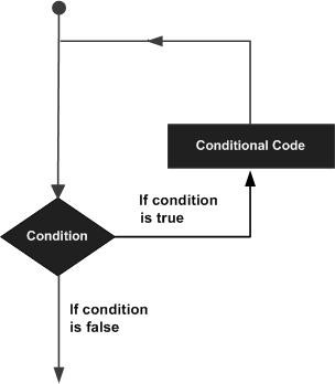
    A loop statement allows us to execute a statement or group of statements multiple times and following is the general form of a loop statement in most of the programming languages −

    Loop Architecture

    MATLAB provides following types of loops to handle looping requirements. Click the following links to check their detail −

    Sr.No.Loop Type & Description
    1while loopRepeats a statement or group of statements while a given condition is true. It tests the condition before executing the loop body.
    2for loopExecutes a sequence of statements multiple times and abbreviates the code that manages the loop variable.
    3nested loopsYou can use one or more loops inside any another loop.

    Loop Control Statements

    Loop control statements change execution from its normal sequence. When execution leaves a scope, all automatic objects that were created in that scope are destroyed.

    MATLAB supports the following control statements. Click the following links to check their detail.

    Sr.No.Control Statement & Description
    1break statementTerminates the loop statement and transfers execution to the statement immediately following the loop.
    2continue statementCauses the loop to skip the remainder of its body and immediately retest its condition prior to reiterating.