System of Linear Algebraic Equations

A system of linear algebraic equations can be represented by the equation:

Equation 1-2. 

where A is an n × n matrix of coefficients, x is an n × 1 vector of unknowns and b an n × 1 vector of constants. Note that the number of equations is equal to the number of the unknowns. A detailed description of the various aspects of the solution of systems of linear equations is provided in Problem 2.4 (Steady-State Material Balances on a Separation Train).

(c) One Nonlinear (Implicit) Algebraic Equation

A single nonlinear equation can be written in the form

Equation 1-3. 

where f is a function and x is the unknown. Additional explicit equations, such as those shown in Section (a), may also be included. Solved problems associated with the solution of one nonlinear equation are presented in Problems 2.1 (Molar Volume and Compressibility Factor from Van Der Waals Equation), 2.9 (Gas Volume Calculations using Various Equations of State), 2.10 (Bubble Point Calculation for an Ideal Binary Mixture), and 2.13 (Adiabatic Flame Temperature in Combustion). These problems should be reviewed before proceeding further. The use of the various software packages for solving single nonlinear equations is demonstrated in solved Problems 4.2 and 5.2 (Calculation of the Flow Rate in a Pipeline). Please study those solved problems as well.

(d) Multiple Linear and Polynomial Regressions

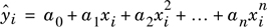
Given a set of data of measured (or observed) values of a dependent variable: y_i versus n independent variables x_1i, x_2i, … x_ni, multiple linear regression attempts to find the “best” values of the parameters a₀, a₁, …a_n for the equation

Equation 1-4. 

where ŷ_i is the calculated value of the dependent variable at point i. The “best” parameters have values that minimize the squares of the errors

Equation 1-5. 

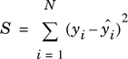
where N is the number of available data points.

In polynomial regression, there is only one independent variable x, and Equation (1-4) becomes

Equation 1-6. 

Multiple linear and polynomial regressions using POLYMATH are demonstrated in detail in solved Problems 3.3 (Correlation of Thermodynamic and Physical Properties of n-Propane) and 3.5 (Heat Transfer Correlations from Dimensional Analysis). The use of Excel and MATLAB for the same purpose is demonstrated respectively in Problems 4.4 and 5.4 (Correlation of the Physical Properties of Ethane). These examples should be studied before proceeding further.

(e) Systems of First-Order Ordinary Differential Equations (ODEs) – Initial Value Problems

A system of n simultaneous first-order ordinary differential equations can be written in the following (canonical) form

Equation 1-7. 

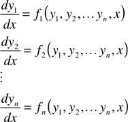
where x is the independent variable and y₁, y₂, … y_n are dependent variables. To obtain a unique solution of n simultaneous first-order ODEs, it is necessary to specify n values of the dependent variables (or their derivatives) at specific values of the independent variable. If those values are specified at a common point, say x₀,

Equation 1-8. 

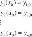
then the problem is categorized as an initial value problem.

The solution of systems of first-order ODE initial value problems is demonstrated in Problems 2.14 (Unsteady-state Mixing in a Tank) and 2.16 (Heat Exchange in a Series of Tanks) where POLYMATH is used to obtain the solution. The use of Excel and MATLAB for systems of first-order ODEs is demonstrated respectively in Problems 4.3 and 5.3 (Adiabatic Operation of a Tubular Reactor for Cracking of Acetone).

(f) System of Nonlinear Algebraic Equations (NLEs)

A system of nonlinear algebraic equations is defined by

Equation 1-9. 

where f is an n vector of functions, and x is an n vector of unknowns. Note that the number of equations is equal to the number of the unknowns. Solved problems in the category of NLEs are Problems 8.11 (Flow Distribution in a Pipeline Network) and 6.6 (Expediting the Solution of Systems of Nonlinear Algebraic Equations). More advanced treatment of systems of nonlinear equations (obtained when solving a constrained minimization problem), is demonstrated along with the use of various software packages in Problems 4.5 and 5.5 (Complex Chemical Equilibrium by Gibbs Energy Minimization).