Momentum Balances

Momentum. The general conservation law also applies to momentum M, which for a mass M moving with a velocity u, as in Fig. 2.13(a), is defined by:

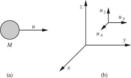
Fig. 2.13 (a) Momentum as a product of mass and velocity; (b) velocity components in the three coordinate directions.

Strangely, there is no universally accepted symbol for momentum. In this text and elsewhere, the symbols M and m (or ) frequently denote mass and mass flow rate, respectively. Therefore, we arbitrarily denote momentum and the rate of transfer of momentum due to flow by the symbols M (“script” M) and , respectively. Momentum is a vector quantity, and for the simple case shown has the direction of the velocity u. More generally, there may be velocity components u_x, u_y, and u_z (sometimes also written as υ_x, υ_y, and υ_z, or as u, υ, and w) in each of the three coordinate directions, illustrated for Cartesian coordinates in Fig. 2.13(b). In this case, the momentum of the mass M has components Mu_x, Mu_y, and Mu_z in the x, y, and z directions.

For problems in more than one dimension, conservation of momentum or a momentum balance applies in each of the coordinate directions. For example, for the basketball shown in Fig. 2.14, momentum Mu_x in the x direction remains almost constant (drag due to the air would reduce it slightly), whereas the upward momentum Mu_z is constantly diminished—and eventually reversed in sign—by the downward gravitational force.

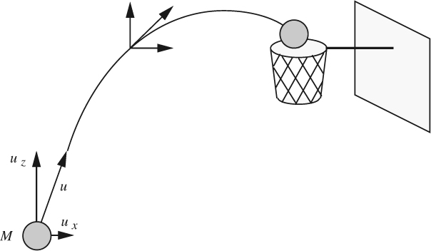
Fig. 2.14 Momentum varies with time in the x and y directions.

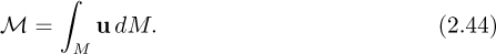
If a system, such as a river, consists of several parts each moving with different velocities u (boldface denotes a vector quantity), the total momentum of the system is obtained by integrating over all of its mass:

Law of momentum conservation. Following the usual law, Eqn. (2.2), the net rate of transfer of momentum into a system equals the rate of increase of the momentum of the system. The question immediately arises: “How can momentum be transferred?” The answer is that there are two principal modes, by a force and by convection, as follows in more detail.

1. Momentum Transfer by a Force

A force is readily seen to be equivalent to a rate of transfer of momentum by examining its dimensions:

In fluid mechanics, the most frequently occurring forces are those due to pressure (which acts normal to a surface), shear stress (which acts tangentially to a surface), and gravity (which acts vertically downwards). Pressure and stress are examples of contact forces, since they occur over some region of contact with the surroundings of the system. Gravity is also known as a body force, since it acts throughout a system.

A momentum balance can be applied to a mass M falling with instantaneous velocity u under gravity in air that offers negligible resistance. Considering momentum as positive downwards, the rate of transfer of momentum to the system (the mass M) is the gravitational force Mg, and is equated to the rate of increase of downwards momentum of the mass, giving:

Note that M can be taken outside the derivative only if the mass is constant. The acceleration is therefore:

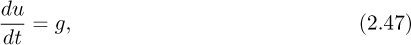
and, although this is a familiar result, it nevertheless follows directly from the principle of conservation of momentum.

Another example is provided by the steady flow of a fluid in a pipe of length L and diameter D, shown in Fig. 2.15. The upstream pressure p₁ exceeds the downstream pressure p₂ and thereby provides a driving force for flow from left to right. However, the shear stress τ_ω exerted by the wall on the fluid tends to retard the motion.

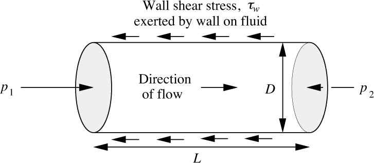
Fig. 2.15 Forces acting on fluid flowing in a pipe.

A steady-state momentum balance to the right (note that a direction must be specified) is next performed. As the system, choose for simplicity a cylinder that is moving with the fluid, since it avoids the necessity of considering flows entering and leaving the system. The result is:

Here, the first term is the rate of addition of momentum to the system resulting from the net pressure difference p₁– p₂, which acts on the circular area πD²/4. The second term is the rate of subtraction of momentum from the system by the wall shear stress, which acts to the left on the cylindrical area πDL. Since the flow is steady, there is no change of momentum of the system with time, and dM/dt = 0. Simplification gives:

which is an important equation from which the wall shear stress can be obtained from the pressure drop (which is easy to determine experimentally) independently of any constitutive equation relating the stress to a velocity gradient.

2. Momentum Transfer by Convection or Flow

The convective transfer of momentum by flow is more subtle, but can be appreciated with reference to Fig. 2.16, in which water from a hose of cross-sectional area A impinges with velocity u on the far side of a trolley of mass M with (for simplicity) frictionless wheels. The dotted box delineates a stationary system within which the momentum Mv is increasing to the right, because the trolley clearly tends to accelerate in that direction. The reason is that momentum is being transferred across the surface BC into the system by the convective action of the jet. The rate of transfer is the mass flow rate m = ρuA times the velocity u, namely:

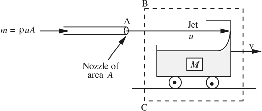
Fig. 2.16 Convection of momentum.

which is again momentum per unit time.

The acceleration of the trolley will now be found by applying momentum balances in two different ways, depending on whether the control volume is stationary or moving. In each case, the water leaves the nozzle of cross-sectional area A with velocity u and the trolley has a velocity υ. Both velocities are relative to the nozzle. The reader should make a determined effort to understand both approaches, since momentum balances are conceptually more difficult than mass and energy balances. It is also essential to perform the momentum balance in an inertial frame of reference—one that is either stationary or moving with a uniform velocity, but not accelerating.

1. Control surface moving with trolley. As shown in Fig. 2.17, the control surface delineating the system is moving to the right at the same velocity υ as the trolley. The observer perceives water entering the system across BC not with velocity u but with a relative velocity (u – v), so that the rate m of convection of mass into the control volume is:

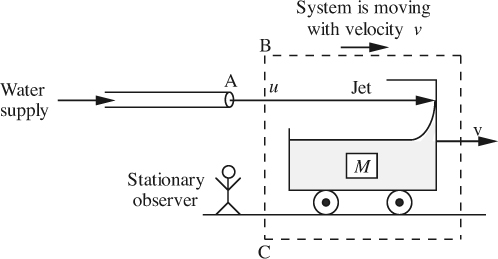
Fig. 2.17 Stationary observer—moving system.

A momentum balance (positive direction to the right) gives:

Note that to obtain the momentum flux, m is multiplied by the absolute velocity u [not the relative velocity (u – v), which has already been accounted for in the mass flux m]. Also, the mass of the system is not constant, but is increasing at a rate given by:

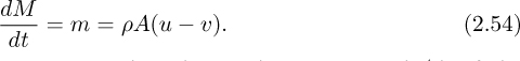
It follows from the last three equations that the acceleration a = dv/dt of the trolley to the right is:

2. Control volume fixed. In Fig. 2.18, the control surface is now fixed in space, so that the trolley is moving within it. Also—and not quite so obviously, that part of the jet of length L inside the control surface is lengthening at a rate dL/dt = υ and increasing its momentum ρALu, and this must of course be taken into account.

A mass balance first gives:

Rate of addition of mass = Rate of increase of mass,

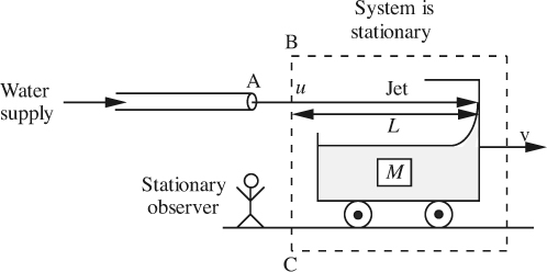
Fig. 2.18 Stationary observer—fixed system.

Likewise, a momentum balance gives:

Rate of addition = Rate of increase.

By eliminating dM/dt between Eqns. (2.56) and (2.57) and rearranging, the acceleration becomes identical with that in (2.55), thus verifying the equivalence of the two approaches:

Example 2.4—Impinging Jet of Water

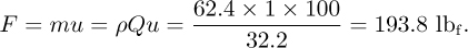
Fig. E2.4 shows a plan of a jet of water impinging against a shield that is held stationary by a force F opposing the jet, which divides into several radially outward streams, each leaving at right angles to the jet. If the total water flow rate is Q = 1 ft³/s and its velocity is u = 100 ft/s, find F (lb_f).

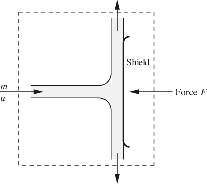
Fig. E2.4 Jet impinging against shield.

Solution

Perform a momentum balance to the right on the system bounded by the dotted control surface. If the mass flow rate is m, the rate of transfer of momentum into the system by convection is mu. The exiting streams have no momentum to the right. Also, the opposing force amounts to a rate of addition of momentum F to the left. Hence, at steady state:

so that:

Example 2.5—Velocity of Wave on Water

As shown in Fig. E2.5(a), a small disturbance in the form of a wave of slightly increased depth D + dD travels with velocity u along the surface of a layer of otherwise stagnant water of depth D. Note that no part of the water itself moves with velocity u—just the dividing line between the stagnant and disturbed regions; in fact, the water velocity just upstream of the front is a small quantity du, and downstream it is zero. If the viscosity is negligible, find the wave velocity in terms of the depth.

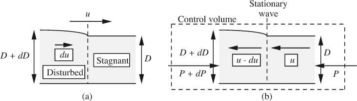
Fig. E2.5 (a) Moving wave front; (b) stationary wave front as seen by observer traveling with wave.

Estimate the warning times available to evacuate communities that are threatened by the following “avalanches” of water:

(a) A tidal wave (closely related to a tsunami²), generated by an earthquake 1,000 miles away, traveling across an ocean of average depth 2,000 ft.

² According to The New York Times of December 27, 2004, a tsunami is a series of waves generated by underwater seismic disturbances. In the disaster of the previous day, the Indian tectonic plate slipped under (and raised) the Burma plate off the coast of Sumatra. The article reported that the ocean floor could rise dozens of feet over a distance of hundreds of miles, displacing unbelievably enormous quantities of water. The waves reached Indonesia, Thailand, Sri Lanka, and elsewhere, causing immense destruction and the eventual loss of more than 225,000 lives.

(b) An onrush, caused by a failed dam 50 miles away, traveling down a river of depth 12 ft that is also flowing towards the community at 4 mph.

Solution

As shown in Fig. E2.5(a), the problem is a transient one, since the picture changes with time as the wave front moves to the right. The solution is facilitated by superimposing a velocity u to the left, as in Fig. E2.5(b)—that is, by taking the viewpoint of an observer traveling with the wave, who now “sees” water coming from the right with velocity u and leaving to the left with velocity u – du.

All forces, flow rates, and momentum fluxes will be based on unit width normal to the plane of the figure. Because the disturbance is small, second-order differentials such as (dD)² and du dD can be neglected. Referring to Fig. E2.5(b), the total downstream and upstream pressure forces are obtained by integration:

A mass balance on the indicated control volume relates the downstream and upstream velocities and their depths (remember that calculations are based on unit width, so D × 1 = D is really an area):

Since the viscosity is negligible, there is no shear stress exerted by the floor on the water above. Therefore, a steady-state momentum balance to the left on the control volume yields:

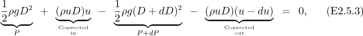
which simplifies to:

Substitution for dD from the mass balance yields the velocity u of the wave:

Note that the wave velocity increases in proportion to the square root of the depth of the water. Another viewpoint is that the Froude number, Fr = u²/gD, being the ratio of inertial (ρu²) to hydrostatic (ρgD) effects, is unity.

The calculations for the water “avalanches” now follow:

(a) Ocean wave: