Mass, Energy, and Momentum Balances

2.1. General Conservation Laws

The study of fluid mechanics is based, to a large extent, on the conservation laws of three extensive quantities:

1. Mass—usually total, but sometimes of one or more individual chemical species.

2. Total energy—the sum of internal, kinetic, potential, and pressure energy.

3. Momentum, both linear and angular.

For a system viewed as a whole, conservation means that there is no net gain nor loss of any of these three quantities, even though there may be some redistribution of them within a system. A general conservation law can be phrased relative to the general system shown in Fig. 2.1, in which can be identified:

1. The system V.

2. The surroundings S.

3. The boundary B, also known as the control surface, across which the system interacts in some manner with its surroundings.

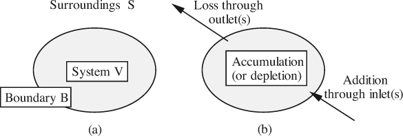
Fig. 2.1 (a) System and its surroundings; (b) transfers to and from a system. For a chemical reaction, creation and destruction terms would also be included inside the system.

The interaction between system and surroundings is typically by one or more of the following mechanisms:

1. A flowing stream, either entering or leaving the system.

2. A “contact” force on the boundary, usually normal or tangential to it, and commonly called a stress.

3. A “body” force, due to an external field that acts throughout the system, of which gravity is the prime example.

4. Useful work, such as electrical energy entering a motor or shaft work leaving a turbine.

Let X denote mass, energy, or momentum. Over a finite time period, the general conservation law for X is:

Nonreacting system

For a mass balance on species i in a reacting system

The symbols are defined in Table 2.1. The understanding is that the creation and destruction terms, together with the superscript i, are needed only for mass balances on species i in chemical reactions, which will not be pursued further in this text.

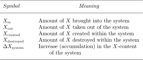
Table 2.1 Meanings of Symbols in Equation (2.1)

It is very important to note that Eqn. (2.1a) cannot be applied indiscriminately, and is only observed in general for the three properties of mass, energy, and momentum. For example, it is not generally true if X is another extensive property such as volume, and is quite meaningless if X is an intensive property such as pressure or temperature.

In the majority of examples in this book, it is true that if X denotes mass and the density is constant, then Eqn. (2.1a) simplifies to the conservation of volume, but this is not the fundamental law. For example, if a gas cylinder is filled up by having nitrogen gas pumped into it, we would very much hope that the volume of the system (consisting of the cylinder and the gas it contains) does not increase by the volume of the (compressible) nitrogen pumped into it!

Equation (2.1a) can also be considered on a basis of unit time, in which case all quantities become rates; for example, ΔX_system becomes the rate, dX_system/dt, at which the X-content of the system is increasing, x_in (note the lower-case “x”) would be the rate of transfer of X into the system, and so on, as in Eqn. (2.2):

2.2. Mass Balances

The general conservation law is typically most useful when rates are considered. In that case, if X denotes mass M and x denotes a mass “rate”m (the symbol  can also be used) the transient mass balance (for a nonreacting system) is:

in which the symbols have the meanings given in Table 2.2.

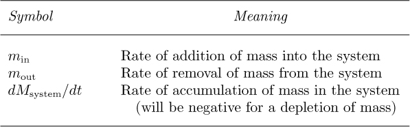
Table 2.2 Meanings of Symbols in Equation (2.3)

The majority of the problems in this text will deal with steady-state situations, in which the system has the same appearance at all instants of time, as in the following examples:

1. A river, with a flow rate that is constant with time.

2. A tank that is draining through its base, but is also supplied with an identical flow rate of liquid through an inlet pipe, so that the liquid level in the tank remains constant with time.

Steady-state problems are generally easier to solve, because a time derivative, such as dM_system/dt, is zero, leading to an algebraic equation.

A few problems—such as that in Example 2.1—will deal with unsteady-state or transient situations, in which the appearance of the system changes with time, as in the following examples:

1. A river, whose level is being raised by a suddenly elevated dam gate downstream.

2. A tank that is draining through its base, but is not being supplied by an inlet stream, so that the liquid level in the tank falls with time.

Transient problems are generally harder to solve, because a time derivative, such as dM_system/dt, is retained, leading to a differential equation.

---

Example 2.1—Mass Balance for Tank Evacuation

The tank shown in Fig. E2.1(a) has a volume V = 1 m³ and contains air that is maintained at a constant temperature by being in thermal equilibrium with its surroundings.

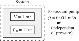
Fig. E2.1(a) Tank evacuation.

If the initial absolute pressure is p₀ = 1 bar, how long will it take for the pressure to fall to a final pressure of 0.0001 bar if the air is evacuated at a constant rate of Q = 0.001 m³/s, at the pressure prevailing inside the tank at any time?

Solution

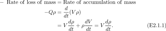
First, and fairly obviously, choose the tank as the system, shown by the dashed rectangle. Note that there is no inlet to the system, and just one outlet from it. A mass balance on the air in the system (noting that a rate of loss is negative) gives:

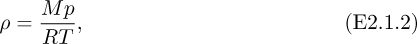
Note that since the tank volume V is constant, dV/dt = 0. For an ideal gas:

so that:

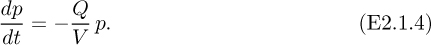
Cancellation of M/RT gives the following ordinary differential equation, which governs the variation of pressure p with time t:

Separation of variables and integration between t = 0 (when the pressure is p₀) and a later time t (when the pressure is p) gives:

The resulting solution shows an exponential decay of the tank pressure with time, also illustrated in Fig. E2.1(b):

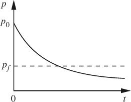
Fig. E2.1(b) Exponential decay of tank pressure.

Thus, the time t_f taken to evacuate the tank from its initial pressure of 1 bar to a final pressure of p_f = 0.0001 bar is:

Problem 2.1 contains a variation of the above, in which air is leaking slowly into the tank from the surrounding atmosphere.

---

Steady-state mass balance for fluid flow. A particularly useful and simple mass balance—also known as the continuity equation—can be derived for the situation shown in Fig. 2.2, where the system resembles a wind sock at an airport. At station 1, fluid flows steadily with density ρ₁ and a uniform velocity u₁ normally across that part of the surface of the system represented by the area A₁. In steady flow, each fluid particle traces a path called a streamline. By considering a large number of particles crossing the closed curve C, we have an equally large number of streamlines that then form a surface known as a stream tube, across which there is clearly no flow. The fluid then leaves the system with uniform velocity u₂ and density ρ₂ at station 2, where the area normal to the direction of flow is A₂.

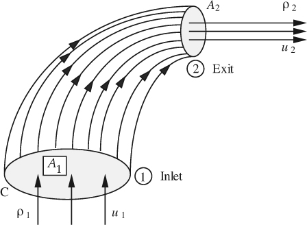
Fig. 2.2 Flow through a stream tube.

Referring to Eqn. (2.3), there is no accumulation of mass because the system is at steady state. Therefore, the only nonzero terms are m₁ (the rate of addition of mass) and m₂ (the rate of removal of mass), which are equal to ρ₁A₁u₁ and ρ₂A₂u₂, respectively, so that Eqn. (2.3) becomes:

which can be rewritten as:

where m (= m₁ = m₂) is the mass flow rate entering and leaving the system.

For the special but common case of an incompressible fluid, ρ₁ = ρ₂, so that the steady-state mass balance becomes:

in which Q is the volumetric flow rate.

Equations (2.4a/b) would also apply for nonuniform inlet and exit velocities, if the appropriate mean velocities u_m1 and u_m2 were substituted for u₁ and u₂. However, we shall postpone the concept of nonuniform velocity distributions to a more appropriate time, particularly to those chapters that deal with microscopic fluid mechanics.

2.3. Energy Balances

Equation (2.1) is next applied to the general system shown in Fig. 2.3, it being understood that property X is now energy. Observe that there is both flow into and from the system. Also note the quantities defined in Table 2.3.

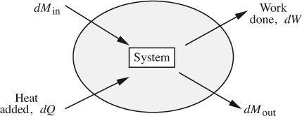
Fig. 2.3 Energy balance on a system with flow in and out.

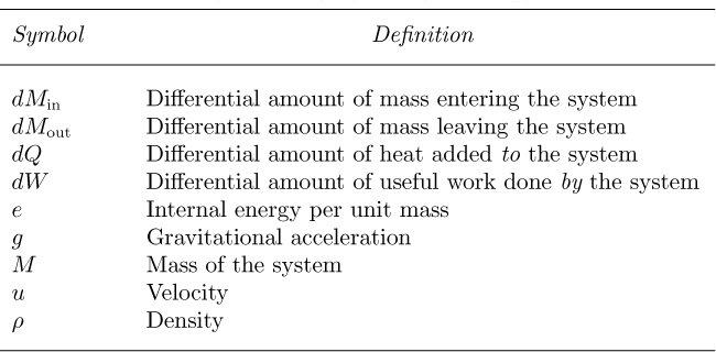
Table 2.3 Definitions of Symbols for Energy Balance

A differential energy balance results by applying Eqn. (2.1) over a short time period. Observe that there are two transfers into the system (incoming mass and heat) and two transfers out of the system (outgoing mass and work). Since the mass transfers also carry energy with them, there results:

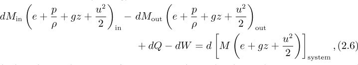
in which each term has units of energy or work. In the above, the system is assumed for simplicity to be homogeneous, so that all parts of it have the same internal, potential, and kinetic energy per unit mass; if such were not the case, integration would be needed throughout the system. Also, multiple inlets and exits could be accommodated by means of additional terms.

Since the density ρ is the reciprocal of υ, the volume per unit mass, e + p/ρ = e + pv, which is recognized as the enthalpy per unit mass. The flow energy term p/ρ in Eqn. (2.6), also known as injection work or flow work, is readily explained by examining Fig. 2.4. Consider unit mass of fluid entering the stream tube under a pressure p₁. The volume of the unit mass is:

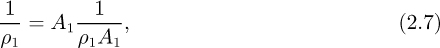
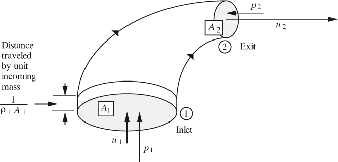
Fig. 2.4 Flow of unit mass to and from stream tube.

which is the product of the area A₁ and the distance 1/ρ₁A₁ through which the mass moves. (Here, the “1” has units of mass.) Hence, the work done on the system by p₁ in pushing the unit mass into the stream tube is the force p₁A₁ exerted by the pressure multiplied by the distance through which it travels:

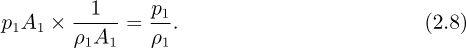
Likewise, the work done by the system on the surroundings at the exit is:

Steady-state energy balance. In the following, all quantities are per unit mass flowing. Referring to the general system shown in Fig. 2.5, the energy entering with the inlet stream plus the heat supplied to the system must equal the energy leaving with the exit stream plus the work done by the system on its surroundings. Therefore, the right-hand side of Eqn. (2.6) is zero under steady-state conditions, and division by dM_in = dM_out gives:

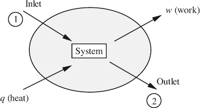
Fig. 2.5 Steady-state energy balance.

in which each term represents an energy per unit mass flowing.

For an infinitesimally small system in which differential changes are occurring, Eqn. (2.10) may be rewritten as:

in which, for example, de is now a differential change, and υ = 1/ρ is the volume per unit mass.

Now examine the increase in internal energy de, which arises from frictional work dF dissipated into heat, heat addition dq from the surroundings, less work pdv done by the fluid. That is: de = dF + dq – pdv. Thus, eliminate the change de in the internal energy from Eqn. (2.11), and expand the term d(pv),

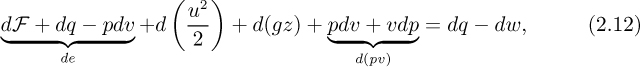
which simplifies to the differential form of the mechanical energy balance, in which heat terms are absent:

For a finite system, for flow from point 1 to point 2, Eqn. (2.13) integrates to:

in which a finite change is consistently the final minus the initial value, for example:

An energy balance for an incompressible fluid of constant density permits the integral to be evaluated easily, giving:

In the majority of cases, g will be virtually constant, in which case there is a further simplification to:

which is a generalized Bernoulli equation, augmented by two extra terms—the frictional dissipation, F, and the work w done by the system. Note that F can never be negative—it is impossible to convert heat entirely into useful work. The work term w will be positive if the fluid flows through a turbine and performs work on the environment; conversely, it will be negative if the fluid flows through a pump and has work done on it.

Power. The rate of expending energy in order to perform work is known as power, with dimensions of ML²/T³, typical units being W (J/s) and ft lb_f/s. The relations in Table 2.4 are available, depending on the particular context.

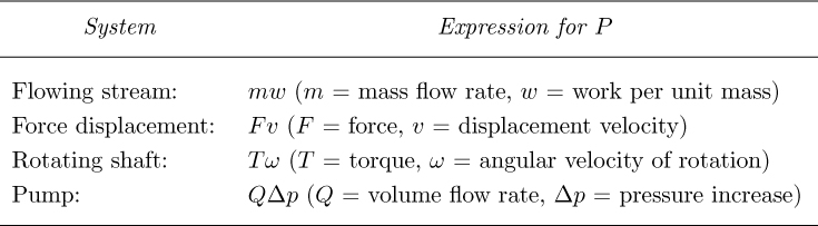
Table 2.4 Expressions for Power in Different Systems

---

Example 2.2—Pumping n-Pentane

Fig. E2.2 shows an arrangement for pumping n-pentane (ρ = 39.3 lb_m/ft³) at 25 °C from one tank to another, through a vertical distance of 40 ft. All piping is 3-in. I.D. Assume that the overall frictional losses in the pipes are given (by methods to be described in Chapter 3) by:

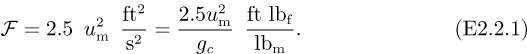
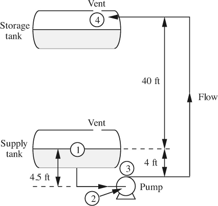
Fig. E2.2 Pumping n-pentane.

For simplicity, however, you may ignore friction in the short length of pipe leading to the pump inlet. Also, the pump and its motor have a combined efficiency of 75%. If the mean velocity u_m is 25 ft/s, determine the following:

(a) The power required to drive the pump.