Physical Properties—Density, Viscosity, and Surface Tension

There are three physical properties of fluids that are particularly important: density, viscosity, and surface tension. Each of these will be defined and viewed briefly in terms of molecular concepts, and their dimensions will be examined in terms of mass, length, and time (M, L, and T). The physical properties depend primarily on the particular fluid. For liquids, viscosity also depends strongly on the temperature; for gases, viscosity is approximately proportional to the square root of the absolute temperature. The density of gases depends almost directly on the absolute pressure; for most other cases, the effect of pressure on physical properties can be disregarded.

Typical processes often run almost isothermally, and in these cases the effect of temperature can be ignored. Except in certain special cases, such as the flow of a compressible gas (in which the density is not constant) or a liquid under a very high shear rate (in which viscous dissipation can cause significant internal heating), or situations involving exothermic or endothermic reactions, we shall ignore any variation of physical properties with pressure and temperature.

Densities of liquids. Density depends on the mass of an individual molecule and the number of such molecules that occupy a unit of volume. For liquids, density depends primarily on the particular liquid and, to a much smaller extent, on its temperature. Representative densities of liquids are given in Table 1.1.² (See Eqns. (1.9)–(1.11) for an explanation of the specific gravity and coefficient of thermal expansion columns.) The accuracy of the values given in Tables 1.1–1.6 is adequate for the calculations needed in this text. However, if highly accurate values are needed, particularly at extreme conditions, then specialized information should be sought elsewhere.

² The values given in Tables 1.1, 1.3, 1.4, 1.5, and 1.6 are based on information given in J.H. Perry, ed., Chemical Engineers’ Handbook, 3rd ed., McGraw-Hill, New York, 1950.

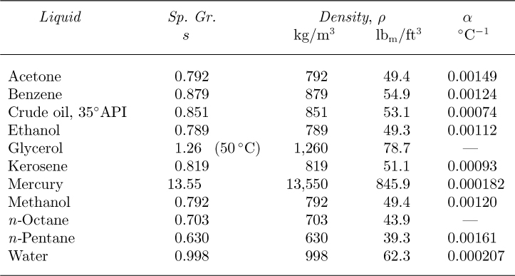
Table 1.1 Specific Gravities, Densities, and Thermal Expansion Coefficients of Liquids at 20 °C

Density. The density ρ of a fluid is defined as its mass per unit volume, and indicates its inertia or resistance to an accelerating force. Thus:

in which the notation “[=]” is consistently used to indicate the dimensions of a quantity.³ It is usually understood in Eqn. (1.5) that the volume is chosen so that it is neither so small that it has no chance of containing a representative selection of molecules nor so large that (in the case of gases) changes of pressure cause significant changes of density throughout the volume. A medium characterized by a density is called a continuum, and follows the classical laws of mechanics—including Newton’s law of motion, as described in this book.

³ An early appearance of the notation “[=]” is in R.B. Bird, W.E. Stewart, and E.N. Lightfoot, Transport Phenomena, Wiley, New York, 1960.

Degrees A.P.I. (American Petroleum Institute) are related to specific gravity s by the formula:

Note that for water, °A.P.I. = 10, with correspondingly higher values for liquids that are less dense. Thus, for the crude oil listed in Table 1.1, Eqn. (1.6) indeed gives 141.5/0.851 – 131.5  35° A.P.I.

Densities of gases. For ideal gases, pV = nRT, where p is the absolute pressure, V is the volume of the gas, n is the number of moles (abbreviated as “mol” when used as a unit), R is the gas constant, and T is the absolute temperature. If M_w is the molecular weight of the gas, it follows that:

Thus, the density of an ideal gas depends on the molecular weight, absolute pressure, and absolute temperature. Values of the gas constant R are given in Table 1.2 for various systems of units. Note that degrees Kelvin, formerly represented by “°K,” is now more simply denoted as “K.”

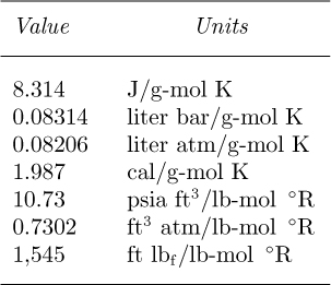
Table 1.2 Values of the Gas Constant, R

For a nonideal gas, the compressibility factor Z (a function of p and T) is introduced into the denominator of Eqn. (1.7), giving:

Thus, the extent to which Z deviates from unity gives a measure of the nonideality of the gas.

The isothermal compressibility of a gas is defined as:

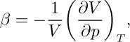
and equals—at constant temperature—the fractional decrease in volume caused by a unit increase in the pressure. For an ideal gas, β = 1/p, the reciprocal of the absolute pressure.

The coefficient of thermal expansion α of a material is its isobaric (constant pressure) fractional increase in volume per unit rise in temperature:

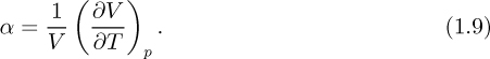
Since, for a given mass, density is inversely proportional to volume, it follows that for moderate temperature ranges (over which α is essentially constant) the density of most liquids is approximately a linear function of temperature:

where ρ₀ is the density at a reference temperature T₀. For an ideal gas, α = 1/T, the reciprocal of the absolute temperature.

The specific gravity s of a fluid is the ratio of the density ρ to the density ρSC of a reference fluid at some standard condition:

For liquids, ρSC is usually the density of water at 4 °C, which equals 1.000 g/ml or 1,000 kg/m³. For gases, ρSC is sometimes taken as the density of air at 60 °F and 14.7 psia, which is approximately 0.0759 lb_m/ft³, and sometimes at 0 °C and one atmosphere absolute; since there is no single standard for gases, care must obviously be taken when interpreting published values. For natural gas, consisting primarily of methane and other hydrocarbons, the gas gravity is defined as the ratio of the molecular weight of the gas to that of air (28.8 lb_m/lb-mol).

Values of the molecular weight M_w are listed in Table 1.3 for several commonly occurring gases, together with their densities at standard conditions of atmospheric pressure and 0 °C.

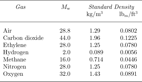
Table 1.3 Gas Molecular Weights and Densities (the Latter at Atmospheric Pressure and 0 °C)

Viscosity. The viscosity of a fluid measures its resistance to flow under an applied shear stress, as shown in Fig. 1.8(a). There, the fluid is ideally supposed to be confined in a relatively small gap of thickness h between one plate that is stationary and another plate that is moving steadily at a velocity V relative to the first plate.

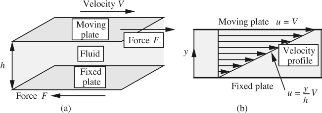
Fig. 1.8 (a) Fluid in shear between parallel plates; (b) the ensuing linear velocity profile.

In practice, the situation would essentially be realized by a fluid occupying the space between two concentric cylinders of large radii rotating relative to each other, as in Fig. 1.1. A steady force F to the right is applied to the upper plate (and, to preserve equilibrium, to the left on the lower plate) in order to maintain a constant motion and to overcome the viscous friction caused by layers of molecules sliding over one another.

Under these circumstances, the velocity u of the fluid to the right is found experimentally to vary linearly from zero at the lower plate (y = 0) to V itself at the upper plate, as in Fig. 1.8(b), corresponding to no-slip conditions at each plate. At any intermediate distance y from the lower plate, the velocity is simply:

Recall that the shear stress τ is the tangential applied force F per unit area:

in which A is the area of each plate. Experimentally, for a large class of materials, called Newtonian fluids, the shear stress is directly proportional to the velocity gradient:

The proportionality constant μ is called the viscosity of the fluid; its dimensions can be found by substituting those for F (ML/T²), A (L²), and du/dy (T^–1), giving:

Representative units for viscosity are g/cm s (also known as poise, designated by P), kg/m s, and lb_m/ft hr. The centipoise (cP), one hundredth of a poise, is also a convenient unit, since the viscosity of water at room temperature is approximately 0.01 P or 1.0 cP. Table 1.11 gives viscosity conversion factors.

The viscosity of a fluid may be determined by observing the pressure drop when it flows at a known rate in a tube, as analyzed in Section 3.2. More sophisticated methods for determining the rheological or flow properties of fluids—including viscosity—are also discussed in Chapter 11; such methods often involve containing the fluid in a small gap between two surfaces, moving one of the surfaces, and measuring the force needed to maintain the other surface stationary.

The kinematic viscosity ν is the ratio of the viscosity to the density:

and is important in cases in which significant viscous and gravitational forces coexist. The reader can check that the dimensions of ν are L²/T, which are identical to those for the diffusion coefficient D in mass transfer and for the thermal diffusivity α = k/ρc_p in heat transfer. There is a definite analogy among the three quantities—indeed, as seen later, the value of the kinematic viscosity governs the rate of “diffusion” of momentum in the laminar and turbulent flow of fluids.

Viscosities of liquids. The viscosities μ of liquids generally vary approximately with absolute temperature T according to:

and—to a good approximation—are independent of pressure. Assuming that μ is measured in centipoise and that T is either in degrees Kelvin or Rankine, appropriate parameters a and b are given in Table 1.4 for several representative liquids. The resulting values for viscosity are approximate, suitable for a first design only.

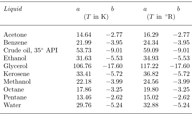
Table 1.4 Viscosity Parameters for Liquids

Viscosities of gases. The viscosity μ of many gases is approximated by the formula:

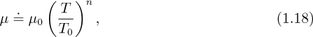
in which T is the absolute temperature (Kelvin or Rankine), μ₀ is the viscosity at an absolute reference temperature T₀, and n is an empirical exponent that best fits the experimental data. The values of the parameters μ₀ and n for atmospheric pressure are given in Table 1.5; recall that to a first approximation, the viscosity of a gas is independent of pressure. The values μ₀ are given in centipoise and correspond to a reference temperature of T₀  273 K  492 °R.

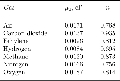
Table 1.5 Viscosity Parameters for Gases

Surface tension.⁴ Surface tension is the tendency of the surface of a liquid to behave like a stretched elastic membrane. There is a natural tendency for liquids to minimize their surface area. The obvious case is that of a liquid droplet on a horizontal surface that is not wetted by the liquid—mercury on glass, or water on a surface that also has a thin oil film on it. For small droplets, such as those on the left of Fig. 1.9, the droplet adopts a shape that is almost perfectly spherical, because in this configuration there is the least surface area for a given volume.